
RUSSIAN JOURNAL OF EARTH SCIENCES, VOL. 18, ES2001, doi:10.2205/2018ES000618, 2018
S. M. Agayan1, Sh. R. Bogoutdinov1,2, R. I. Krasnoperov1
1The Geophysical Center of RAS, Moscow, Russia
2Institute of Physics of the Earth of RAS, Moscow, Russia
Discrete Mathematical Analysis (DMA) is a new approach to data analysis that is being developed at the Geophysical Center of the Russian Academy of Sciences. Multiple papers, which have been published earlier, are mainly devoted to applied research and solving specific problems in various areas of the Earth's sciences, such as detection of geophysical anomalies, monitoring of geophysical processes, seismic zoning, etc. The goal, which the authors pursue in this paper, is, to a certain degree, opposite – to give a formal mathematical description of principles that form the basis of DMA.
|
| Figure 1 |
Data mining in natural sciences can be very schematically presented as follows (Figure 1). Nowadays the analysis and processing of data are performed mainly by using such classical methods as statistical analysis, time-frequency signal analysis, wavelet analysis, fractal analysis and mathematical morphology, which currently gains popularity.
For all the advantages, most of them have excessive robustness because of their mathematical origin. This means that the object, which is being studied (more likely, its model), has to meet certain preliminary criteria (stationarity, normalcy, regularity, etc.). If they fail to meet them, then problems may occur. Previously they were solved by model's simplification.
In recent times due to the development of computational tools more gentle and undemanding approaches have been introduced (combinatory exhaustive search, imitational modelling, neural networks, etc.)
 |
| Figure 2 |
The presented scheme (Figure 1) does not include a researcher while his role is important even in case of a firm theory (e.g. during the discussion and interpretation of results) and completely essential in other cases. The more accurate will be the scheme, shown in Figure 2. It represents the situation in geology and geophysics (which is particularly close to the authors' practice): the researcher's role in this area is extremely important, since data and knowledge tend to be irregular and ill-defined.
In comparison to any formal apparatus an experienced researcher is more accurate in detection of anomalies in low-dimensional physical fields; transit from local level to the global one for achieving interpretational unity; in recognition of signals of any desired form within short fragments of records; etc. But he fails to deal with large dimensions and volume. For that reason, the task of learning the computer to analyze data as a researcher becomes particularly topical.
The fact that human thinks and operates not in numbers but in fuzzy concepts was primarily considered while solving the problem. Therefore, the technical basis of our modelling along with the classical mathematics was formed with fuzzy mathematics and directly through it with fuzzy logic [Zadeh, 1965].
The authors presume that the researcher's advantage in data analysis over the formal methods is explained by a man's flexible and adaptive perception of fundamental features of proximity, continuity, connectivity, trend, etc., because these particular features, like a "construction set", form all the algorithms for data analysis. The more thoroughly the features are modelled, the more comprehensive the "construction set" is. It is the reason why there should be plenty of continuities, connectivities, trends, etc.
The resulting solution is a new approach to data analysis that is, being researcher-oriented, falls in between robust mathematical methods and gentle combinatory. It is DMA [Gvishiani et al., 2010].
Discrete mathematical analysis (DMA) is a series of algorithms for processing of discrete data, unified by common formal basis: numeric fuzzy comparison, measure of proximity in discrete spaces, discrete limit. The idea of DMA is based on the construction of discrete analogues of classical mathematical analysis concepts: limit, continuity, smoothness, connectivity, monotonicity, extremum, etc.
Thus, our way is to implement the classical continuous mathematics, substituting its fundamental basis with fuzzy models of their discrete analogues.
 |
| Figure 3 |
Referring to scheme (Figure 3), let's presume that we know what large–small is, thus we can construct the following mathematical concepts:
and concepts of data analysis:
For construction of DMA and particularly for implementation of the presented scheme the ordinary sets and Boolean logic are not sufficient: Boolean features are internally disjoint (robust), what leads to modeling emasculation. Conceptual features have to be continuous (gentle) and thus, fuzzy.
Fuzzy mathematics = fuzzy sets + fuzzy logic.
Fuzzy mathematics is an appropriate link (interface) between a researcher and a computer.
Definition 1. Fuzzy set $A$ $\equiv$ is set of pairs $(x,\mu_A(x))$, where $x$ – point within universal $X$, and $\mu_A(x)$ – degree of membership $x$ to $A$.
We adopt two concepts from fuzzy mathematics:
Commonly in DMA $X$ is the range of definition of a data record, field or process. Any feature of theirs is manifested within $X$ to various degrees and in this aspect, it can be considered as a gentle structure within $X$.
From this perspective, in order to set up the scheme in Figure 3 one should answer a question, what "large" is, and what "small" is.
Given: $A=\displaystyle{\{ (a_k,\omega_k)|_{k=1}^K,\omega_k>0\}}$ – a finite numerical collection with weights.
Definition 2. Measure of maximality ${\rm mesmax}, _A(x)$ (minimality ${\rm mesmin} \, _A (x)$) is a fuzzy structure within $\mathbb{R}$, that answers the question: "To what measure
Measure of extremality $\equiv$ (Measure of maximality) $\vee$ (Measure of minimality)
Informal interpretation for functions: ${\rm mesmax} \, f(x)$ shows to what degree the value of function $f$ in a point $x$ is large. The same is for ${\rm mesmin} \, f(x)$.
\begin{eqnarray*} f:X \rightarrow \mathbb{R}, \quad {\rm mesmax} \, f(x)={\rm mesmax} \, _{\textrm{Im}\, f} f(x) \end{eqnarray*} \begin{eqnarray*} \quad\quad\quad\quad\quad{\rm mesmin} \, f(x)={\rm mesmin} \, _{\textrm{Im}\, f} f(x) \end{eqnarray*}There are four constructions for measures in DMA. The most transparent is "fuzzy comparison"
In many cases the conventional linear measure of greatness of one number over another as their difference appears to be too coarse.
Definition 3. Fuzzy comparison $n(a,b)$ for nonnegative numbers $a,b\in \mathbb{R}^+$ defines the level of greatness of "$b$" over "$a$":
\begin{eqnarray*} n(a,b)={\rm mes} \,(a < b)\in [-1,1]. \end{eqnarray*}Example 1. $\displaystyle{n(a,b)=\frac{b-a}{\max(a,b)}}$. Two pairs of numbers are given $(5,10)$ and $(70,75)$. The conventional difference for them is equal, whereas the fuzzy comparison is varying:
\begin{eqnarray*} \begin{array}{l} {\rm mes} \,(5 < 10)=n(5,10)=\frac{5}{10}=\frac{1}{2} \newline {\rm mes} \,(70 < 75)=n(70,75)=\frac{5}{75}=\frac{1}{15} \end{array} \end{eqnarray*}which seems more natural $($a five-year-old child differs greatly from a ten-year-old one, than a seventy-year-old man from a seventy-five-year-old one$)$.
Every fuzzy comparison defines the measures of extremeness, for example by means of the binary method:
\begin{eqnarray*} {\rm mesmax} \, _A x = \displaystyle{\frac{\sum \omega _i n(a_i,x)}{\sum \omega _i} \in [-1,1]} \end{eqnarray*} \begin{eqnarray*} {\rm mesmin} \, _A x = \displaystyle{\frac{\sum \omega _i n(x,a_i)}{\sum \omega _i} \in [-1,1]} \end{eqnarray*}Thus, we have an answer for the question: "What is large and what is small?"
Definition 4. The element $x$ is large $($small$)$ modulo $A$, if ${\rm mesmax} \,_A x \ge 0.5$ $({\rm mesmin} \,_A x \ge 0.5)$.
Proximity measures are constructed using the measures of minimality. Let us give two constructions.
$\bullet$ 1st construction: $dX$ is an assembly of all non-trivial distances in the space $X$. For points $x$ and $y$ the following problem is solved: "To what degree the distance $d(x,y)$ between them is small amongst the others?". The answer is $\delta _x(y)$.
\begin{eqnarray*} dX=\{d(\bar{x},\bar{y}): \bar{x} \ne \bar{y} \in X \} \end{eqnarray*} \begin{eqnarray*} \delta _x(y)=n(d(x,y),dX)= \displaystyle{\frac{\sum _{\bar{y} \ne x}n(d(x,y),d(\bar{x},\bar{y})}{|X|(|X|-1)}} \end{eqnarray*}$\bullet$ 2nd construction: $dX(x)$ is an assembly of distances from $x$ to other points from $X$. Further the same.
\begin{eqnarray*} dX(x)=\{d(x,\bar{y}): \bar{y} \in X-x \} \end{eqnarray*} \begin{eqnarray*} \delta _x(y)=n(d(x,y),dX(x))= \displaystyle{\frac{\sum _{\bar{y} \ne x}n(d(x,y),d(x,\bar{y}))}{|X|-1}} \end{eqnarray*} |
| Figure 4 |
Example 2.Application of the 2nd construction (see Figure 4).
NB: The denser is the space at a point (Figure 4), the lesser is the radius of the red circle. In other words, such a circle can be considered as the criteria of density (irreducibility) of the space at a point. Let us give a general definition:
Definition 5. For a subset $A \subset X$ density $P_A(x)$ is the function of membership within $X$ for the fuzzy concept "proximity (irreducibility) to $A$ in $X$": value $P_A(x)$ expresses in the scale $[0,1]$ the degree of proximity (irreducibility) of point $x$ to subset $A$ within the space $(X,d)$
Let us give two constructions:
$\bullet$ 1st construction continues the concept of proximity measures from two points to a subset and a point: if $d(\cdot,A)$ is a variant of the distance to $A$ in $X$, $d(X,A)=\{d(x,A):x \in X \}$, then
\begin{eqnarray*} P_A (x)= {\rm mesmin} \, _{d(X,A)}d(x,A) \end{eqnarray*}$\bullet$ 2nd construction implements "dense – large presence of proximate points". Let $r > 0, D_A (x,r)=\{a \in A:d(a,x) \le r \}$, $ D_A (X,r)=\{D_A(y,r),y \in X \}$. Then
\begin{eqnarray*} \begin{array}{l} P_A(x) = {\rm mesmax} \, _{|D_A(X,r)|} |D_A(x,r)|. \end{array} \end{eqnarray*}Let $(X,d)$ be the finite metric space, $P_X(\cdot)$ is the chosen density model within it, $P(X)=\{P_X (x): x\in X\}$.
Definition 6. The point $x^*$ is dense in $X$, if ${\rm mesmax} \, _{P(X)} P_X(x^*) \ge 0.5$
 |
| Figure 5 |
Example 3. Red color denotes dense points (see Figure 5).
DMA defines clusters informally as continuous regions of the initial space with a relatively high density of points that are separated from other similar ones by regions with relatively low density. The basis of the rigorous formalization of clusterness forms the abovementioned conjunction:
Clusterness $\equiv$ density $+$ connectivity.
Let us consider connectivity: the measure of density $\delta$ and density threshold $\alpha$ are chosen.
Definition 7. $A$ – $\alpha$-$\delta$-connected, if $\forall x,y \in X$ there is a chain $z_1,\ldots,z_n$ with $x=z_1$ and $y=z_n$, for which $\delta _{z_i} (z_{i+1})\ge \alpha$, $i=1,\ldots,n-1$.
This definition implements "connectivity as ability to transfer through proximate points".
Definition 8. $A$ – $\alpha$-$\delta$-cluster, if $\underset{x \in A}{\min} P_A (x)\ge \beta$ $\wedge$ $A$ – $\alpha$-$\delta$-connected.
DMA-clustering (density + connectivity) is more realistic, than traditional, such as clustering in noisy spaces. It includes two stages:
 |
| Figure 6 |
Example 4. Figure 6 demonstrates DMA-clustering with respect to vertical view on density $($the densest is in the bottom of the hills$)$: Figure 6a - initial set; Figure 6b - result of the 1st stage; Figure 6c - result of the 2nd stage.
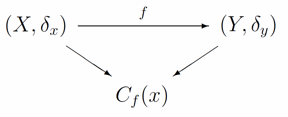
Discrete continuity is in the focus in the DMA, since it is closely associated with discontinuity (one of the manifestations of anomaly). Let us consider the following approach: let $f$ be the mapping of finite metric spaces $X$ and $Y$, which transfers point $x\in X$ into point $y\in Y$:
\begin{eqnarray*} f:X\rightarrow Y \quad X \ni x \overset{f}{\rightarrow} y \in Y. \end{eqnarray*}The abovementioned fuzzy comparisons and measures of proximity allow formalizing the concept of continuity $f$ in point $x$: any pair of proximity measures $\delta _x$ at point $x$ within $X$, $\delta _y$ at point $y$ within $Y$ allow to implement the formulated earlier logic of continuity (proximate to proximate) of mapping $f$ and obtain fuzzy measure of continuity $C_f(x)$ of mapping $f$ at point $x$:
Definition 9.
\begin{eqnarray*} D(x) = \{\bar{x} \in X: \delta _x (\bar{x}) \ge 0.5 \} \end{eqnarray*} \begin{eqnarray*} D(y) = \{\bar{y} \in Y: \delta _y (\bar{y}) \ge 0.5 \} \end{eqnarray*} \begin{eqnarray*} \displaystyle{C_f(x) = \frac{|\bar{x} \in D(x): f(\bar{x}) \in D(y)|}{|D(x)|}} \end{eqnarray*} |
| Figure 7 |
Example 5. In Figure 7 red color shows the points, where mapping $f$ has a low measure of discrete continuity $($high measure of anomaly$)$
Let there be given a series $x \sim \left(x(t_i)|_0^N\right)$, $t_i=a+ih$. $h=\frac{b-a}{N}$, $t_0=a$, $t_N=b$
Definition 10. Let's specify limitations $x|_{[a,t_i]}$ and $x|_{[t_i,b]}$, respectively left and right parts of $x$ at node $t_i$ and denote them respectively as $Lx(t_i)$ and $Rx(t_i)$.
Series $x$ increases (decreases) at node $t_i$, if $Lx(t_i)\le Rx(t_i)$ ($Rx(t_i)\le Lx(t_i)$).
These inequations are modeled differently by fuzzy comparisons. Fuzzy measure also assigned differently. Let us consider one of the possible schemes of such modeling. Let $\delta _{t_i}^{-}(t_j)$ and $\delta _{t_i}^{+}(t_j)$ be the one-sided weights at node $t_i$:
\begin{eqnarray*} \begin{array}{c} \displaystyle{\delta _{t_i}^{-}(t_j)=\frac{t_j -a+h}{t_i -a+h}} \quad\quad\quad\quad \displaystyle{\delta _{t_i}^{+}(t_j)=\frac{b+h-t_j}{b+h-t_i}} \end{array} \end{eqnarray*}and
\begin{eqnarray*} \displaystyle{\textrm{gr}^{-}x(t_i)=\frac{\sum x(t_j)\delta _{t_i}^{-}(t_j)}{\sum \delta _{t_i}^{-}(t_j)}, t_j \in [a,t_i]} \end{eqnarray*} \begin{eqnarray*} \displaystyle{\textrm{gr}^{+}x(t_i)=\frac{\sum x(t_j)\delta _{t_i}^{+}(t_j)}{\sum \delta _{t_i}^{+}(t_j)}, t_j \in [t_i,b]} \end{eqnarray*}Definition 11.
The difference of such trends from the ordinary ones is that they intersect covering each other. Their intersection is the fuzzy extremum. Choosing the only candidate for the fuzzy extremum within it is a separate task, which has been solved within DMA.
 |
| Figure 8 |
Example 6. Figure 8 demonstrates the results of definition of trends and fuzzy extremums in different situations. Red color shows the zones of monotonous increase, green – monotonous decrease, cyan – fuzzy extremums.
So, we have answered all the main problems of data analysis and hence formed its variant. Many of them are "able to shoot and engaged in active combat". But, for example, the block "continuous–discontinuous" is not very convenient for detecting real anomalies, since they are much wider and more complicated.
This task is solved by the system for monitoring of dynamic processes that was developed within the DMA framework. A dynamic process is defined as number of time series of arbitrary nature. Monitoring includes the analysis of activity measures [Agayan et al., 2016] of separate time series with consecutive assessment of the dynamic processes' anomality in general. Measure of activity is the formalization of the fuzzy and multivalent concept of a time series activity. Any time series may be connected with a number of measures of activity that implement various views on its activity.
 |
| Figure 9 |
For automated assessment of geomagnetic activity level within a region, where a separate geomagnetic observatory is located; or for assessment of geomagnetic conditions within a given region using data from a network of observatories; or for global assessment of magnetic disturbances within the Earth, a new indicator has been introduced. It is based on the value of the measure of anomality $\mu$ of a magnetometer data at a given moment (time interval). This indicator allows to measure the level of geomagnetic activity at various observatories on a single scale regardless the amplitude of disturbances, common to a given observatory. This amplitude depends on the latitude where an observatory is located. The largest amplitudes of geomagnetic disturbances are typical for auroral regions. The indicator $\mu$ to a certain extent is the analog of the traditional $Kp$-index (Figure 9) [Love and Remick, 2007]. But its widely known disadvantage is its extremely large 3-hour time interval, within which the index is calculated. Moreover, the calculation of $Kp$-index requires preliminary elimination of regular daily variation from magnetograms, which is highly labor-consuming and causes delays. Nowadays there is a demand of operative geomagnetic indices, calculated with a 1-minute interval and provided in the internet in quasi-real mode. The proposed indicator $\mu$ is aimed to overcome the disadvantages of the traditional $Kp$-index. Calculation of $\mu$ is algorithmized and may be executed in operative and automated mode with the same frequency as the initial data are acquired.
Let's consider an example of geophysical monitoring of geomagnetic nature. Measures of activity $\mu$ in this case play the same role as the indices of geomagnetic activity. Let us compare $\mu$ with a widely known $Kp$-index.
 |
| Figure 10 |
The magnetic conditions in the network within 3 hours according to $Kp$-index and $\mu$ are presented in Figure 10 respectively horizontally and vertically.
Using the Kolmogorov's mean a new system of coordinates is constructed. In its first (third) quadrant interesting (uninteresting) events, according to $Kp$-index and $\mu$, are located. The fourth quadrant contains events, which are interesting according to $Kp$-index and uninteresting according to $\mu$. The opposite quadrant is untrivial, it contains events, which are interesting according to $\mu$ and uninteresting according to $Kp$-index (Figure 10).
 |
| Figure 11 |
Indeed, let's consider one of the events from the second quadrant and compare them with the corresponding intervals of the magnetic records, registered at stations that perform monitoring (Figure 11).
It is apparent that within the first hour all of the considered stations register a certain event. It was detected by the index based on measure of activity, and missed by the standard $Kp$-index.
The goal the authors pursued in this paper is to give a brief formal mathematical description of the Discrete Mathematical Analysis (DMA) approach. We formally described the basis of mathematical concepts which form the apparatus of DMA: proximate–remote, dense–non-dense, continuous–discontinuous, clusters, and trends. A more detailed description and examples of DMA-application for geological and geophysical tasks (monitoring of geophysical processes, seismic zoning, analysis of magnetograms) can be found in the following
papers: [Agayan et al., 2014; 2016], [Bogoutdinov et al., 2010], [Gvishiani et al., 2008a; 2008b; 2010; 2013a; 2013b; 2016], [Mikhailov et al., 2003], [Sidorov et al., 2012], [Soloviev et al., 2012a; 2012b; 2013; 2016], [Zelinskiy et al., 2014], [Zlotnicki et al., 2005].
Agayan, S., Sh. Bogoutdinov, M. Dobrovolsky (2014), Discrete Perfect Sets and their application in cluster analysis, Cybernetics and Systems Analysis, 50, no. 2, p. 176–190, https://doi.org/10.1007/s10559-014-9605-9.
Agayan, S., Sh. R. Bogoutdinov, A. Soloviev, et al. (2016), The Study of Time Series Using the DMA Methods and Geophysical Applications, Data Science Journal, 15, p. 1–15, https://doi.org/10.5334/dsj-2016-016.
Bogoutdinov, Sh. R., A. D. Gvishiani, S. M. Agayan, A. A. Soloviev, E. Kihn (2010), Recognition of disturbances with specified morphology in time series. Part 1: Spikes on Magnetograms of the Worldwide INTERMAGNET Network, Physics of the Solid Earth, 46, no. 11, p. 1004–1016, https://doi.org/10.1134/S1069351310110091.
Gvishiani, A. D., S. M. Agayan, Sh. R. Bogoutdinov (2008), Fuzzy recognition of anomalies in time series, Doklady Earth Sciences, 421, no. 1, p. 838–842, https://doi.org/10.1134/S1028334X08050292.
Gvishiani, A. D., S. M. Agayan, Sh. R. Bogoutdinov, A. A. Soloviev (2010), Discrete mathematical analysis and applications geology and geophysics, Bulletin of KRAESC. Earth Sciences, no. 10, p. 109–125.
Gvishiani, A. D., S. M. Agayan, Sh. R. Bogoutdinov, J. Zlotnicki, J. Bonnin (2008), Mathematical methods of geoinformatics. III. Fuzzy comparisons and recognition of anomalies in time series, Cybernetics and System Analysis, 44, no. 3, p. 309–323, https://doi.org/10.1007/s10559-008-9009-9.
Gvishiani, A. D., M. N. Dobrovolsky, S. Agayan, B. Dzeboev (2013), Fuzzy-based clustering of epicenters and strong earthquake-prone areas, Environmental Engineering and Management Journal, 12, no. 1, p. 1–10.
Gvishiani, A. D., B. Dzeboev, S. M. Agayan (2013), A new approach to recognition of the strong earthquake-prone areas in the Caucasus, Izvestiya, Physics of the Solid Earth, 49, no. 6, p. 747–766, https://doi.org/10.1134/S1069351313060049.
Gvishiani, A. D., A. Soloviev, R. Krasnoperov, et al. (2016), Automated Hardware and Software System for Monitoring the Earth's Magnetic Environment, Data Science Journal, 15, no. 18, p. 1–24, https://doi.org/10.5334/dsj-2016-018.
Love, J., K. J. Remick (2007), Magnetic indices In: Gubbins, D and Herrero-Bervera, E (eds.) Encyclopedia of Geomagnetism and Paleomagnetism, 711–713 pp., Springer, New York.
Mikhailov, V., et al. (2003), Application of artificial intelligence for Euler solutions clustering, Geophysics, 68, no. 1, p. 168–180, https://doi.org/10.1190/1.1543204.
Sidorov, R. V., A. A. Soloviev, Sh. R. Bogoutdinov (2012), Application of the SP algorithm to the INTERMAGNET magnetograms of the disturbed geomagnetic field, Izvestiya, Physics of the Solid Earth, 48, no. 5, p. 410–414, https://doi.org/10.1134/S1069351312040088.
Soloviev, A., S. M. Agayan, Sh. R. Bogoutdinov (2016), Estimation of geomagnetic activity using measure of anomalousness, Annals of Geophysics, 59, no. 6, p. 1–17, https://doi.org/10.4401/ag-7116.
Soloviev, A., Sh. R. Bogoutdinov, A. D. Gvishiani, R. Kulchinskiy, J. Zlotnicki (2013), Mathematical Tools for Geomagnetic Data Monitoring and the INTERMAGNET Russian Segment, Data Science Journal, 12, p. WDS114–WDS119, https://doi.org/10.2481/dsj.WDS-019.
Soloviev, A., A. Chulliat, Sh. R. Bogoutdinov, et al. (2012), Automated recognition of spikes in 1 Hz data recorded at the Easter Island magnetic observatory, Earth, Planets and Space, 64, no. 9, p. 743–752, https://doi.org/10.5047/eps.2012.03.004.
Soloviev, A. A., S. M. Agayan, A. D. Gvishiani, et al. (2012), Recognition of disturbances with specified morphology in time series. Part 2: Spikes on 1-s magnetograms, Izvestiya, Physics of the Solid Earth, 48, no. 5, p. 395–409, https://doi.org/10.1134/S106935131204009X.
Zelinskiy, N. R., N. G. Kleimenova, O. V. Kozyreva, S. M. Agayan, Sh. R. Bogoutdinov, A. A. Soloviev (2014), Algorithm for recognizing Pc3 geomagnetic pulsations in 1-s data from INTERMAGNET equatorial observatories, Izvestiya, Physics of the Solid Earth, 50, no. 2, p. 240–248, https://doi.org/10.1134/S106935131402013X.
Zadeh, L. A. (1965), Fuzzy sets, Information Control, 8, no. 3, p. 338–353, https://doi.org/10.1016/S0019-9958(65)90241-X.
Zlotnicki, J., J.-L. LeMouel, A. D. Gvishiani, et al. (2005), Automatic fuzzy-logic recognition of anomalous activity on long geophysical records. Application to electric signals associated with the volcanic activity of la Fournaise volcano (Reunion Island), Earth and Planetary Science Letters, 234, no. 1–2, p. 261–278, https://doi.org/10.1016/j.epsl.2005.01.040.
INTERMAGNET, (1991), International Real-time Magnetic Observatory Network web-page, WDCS, Paris, .
WDC, (1957), World Data Center for Geomagnetism, Kyoto, WDCS, Kyoto, .
Received 21 January 2018; accepted 26 February 2018; published March 2018.

Citation: Agayan S. M., Sh. R. Bogoutdinov, R. I. Krasnoperov (2018), Short introduction into DMA, Russ. J. Earth Sci., 18, ES2001, doi:10.2205/2018ES000618.
Copyright 2018 by the Geophysical Center RAS.