 |
| Figure 1 |
 |
| Figure 2 |
RUSSIAN JOURNAL OF EARTH SCIENCES, VOL. 17, ES4001, doi:10.2205/2017ES000604, 2017
A. A. Lushnikov1,2, V. A. Zagaynov2, Yu. S. Lyubovtseva1
1Geophysical Center of Russian Academy of Science, Moscow, Russia
2National Research Nuclear University MEPhI, Moscow, Russia
This paper overviews the observations of aerosol events in the atmosphere in view of a simple linear model of the formation of nanoaerosols in the atmosphere. The model includes three input functions: the rate of formation of the smallest (1.5 nm in diameter) particles by nucleation, the particle growth rate, and the coagulation sink of newly born particles. Neglecting the self-coagulation of newly born particles (this process is slow) simplifies the growth equation describing time evolution of the particle size distribution. This equation becomes linear and is solved exactly. The most remarkable feature of our consideration is that the particle size distribution can be presented as a superposition of different growth regimes. In particular, if the source-enhanced particle growth is combined with the free regime, the latter produces a running wave that moves to the right along the size axis giving the picture very similar to that observed during the nucleation events. The source-enhanced regime alone can also produce the wave moving to the right but the picture is much less expressive. Another possibility discussed here is an abrupt change in the particle source intensity because of increasing the condensation sink. The source stops producing fresh particles and the whole particle distribution begins to shift to the right along the particle size axis. Similar picture is observed if the nucleation process goes at nighttime and stops at daytime. In this case the particles accumulated during the night grow in the free regime at daytime by condensing the low volatile substances formed in photochemical reactions. The particle size spectra are found for different sets of the parameters. Possible scenarios of nucleation bursts are discussed.
Regular production of nonvolatile species of anthropogenic or natural origin in the atmosphere eventually leads to their nucleation, formation of tiny aerosol particles and their subsequent growth. Thus formed aerosol is able to inhibit the nucleation process because of condensation of nonvolatile substances onto the surfaces of newly born particle surfaces. This process is referred to as the nucleation burst [Friedlander, 1977, 1983].
The dynamics of atmospheric nucleation bursts possesses its own specifics, in particular, the particle production and growth is suppressed mainly by preexisting aerosols rather than freshly formed particles of nucleation mode [Kerminen et al., 2001; Dal Maso et al., 2002]. In many cases the nucleation bursts have a heterogeneous nature. The smallest (undetectable) particles accumulated during nighttime begin to grow at daytime because of sunlight driven photochemical cycles producing low volatile (but not nucleating) substances that are able to activate the aerosol particles [Kulmala et al., 2006]. Stable sulfate clusters [Kulmala et al., 2000] can serve as heterogeneous embryos provoking the nucleation bursts.
The nucleation bursts were regularly observed in the atmospheric conditions and were shown to serve as an essential source of cloud condensation nuclei [Kulmala, 2003; Kulmala et al., 2004a; Kulmala and Tammet, 2007].
In this paper we apply a simple linear model for analyzing the nature of the atmospheric nucleation bursts.
Now it becomes more and more evident that the nucleation bursts in the atmosphere can contribute substantially to CCN production and can thus affect the climate and weather conditions on our planet (see e.g., [Spracklen et al., 2006 and references therein]. Existing at present time opinion connects the nucleation bursts with additional production of nonvolatile substances that can then nucleate producing new aerosol particles, and/or condense onto the surfaces of newly born particles, foreign aerosols, or on atmospheric ions. The production of nonvolatile substances, in turn, demands some special conditions to be fulfilled imposed on the emission rates of volatile organics from vegetation, current chemical content of the atmosphere, rates of stirring and exchange processes between lower and upper atmospheric layers, presence of foreign aerosols [accumulation mode, first of all) serving as condensational sinks for trace gases and the coagulation sinks for the particles of nucleation mode, the interactions with air masses from contaminated or clean regions [Kerminen et al., 2000; Adams and Seinfeld, 2003; Boy and Kulmala, 2002; Kulmala, 2003; Kulmala et al., 2004a; 2004b; 2004c; Kulmala et al., 2005; Kerminen et al., 2004a, 2004b; Dal Maso et al., 2005]. Such a plethora of very diverse factors most of which have a stochastic nature prevents direct attacks on this effect. A huge amount of field measurements of nucleation bursts dynamics appeared during the last decade (see [Kavouras et al., 1998; Kerminen et al., 2000; Kulmala et al., 2001; Aalto et al., 2001; Janson et al., 2001; O'Dowd et al., 2003; Boy and Kulmala, 2002; Boy et al., 2003; Kulmala, 2003; Kulmala et al., 2004a; 2004b; 2004c; Dal Maso et al., 2005; Lyubovtseva et al., 2005; Kerminen et al., 2004a; 2004b; Stolzenberg et al., 2005].
The attempts of modelling this important and still enigmatic process also appeared rather long ago. Here we avoid the long history of this problem and cite only the last models appeared in the XXI century: [Barret and Clement, 1991; Clement and Ford, 1999; Clement et al., 2006; Adams et al., 2002; Korhonen et al., 2003; Lehtinen and Kulmala, 2003; Easter et al., 2004; Anttila et al., 2004; Korhonen et al., 2004; Grini et al., 2005; Lushnikov et al., 2013a, 2013b; Lushnikov et al., 2014; Elperin et al., 2013; Stolzenberg et al., 2005; Spracklen et al., 2006]. The extensive earlier citations can be found in the above listed papers. All models (with no exception) start from commonly accepted point of view that the chemical reactions of trace gases are responsible for the formation of nonvolatile precursors which then give the life to subnano- and nanoparticles in the atmosphere. In their turn, these particles are considered as active participants of the atmospheric chemical cycles leading to the particle formation [Hoffmann et al., 1997; Griffin et al., 1999; Janson et al., 2001; Griffin et al., 2002]. Hence, any model of nucleation bursts included (and includes) coupled chemical and aerosol blocks. This coupling leads to strong nonlinearities which means that all intra-atmospheric chemical processes (not all of which are, in addition, firmly established) are described by a set of nonlinear equations, and there is not an assurance that we know all the participants of the chemical cycles leading to the production of low volatile gas constituents that then convert to the tiniest aerosol particles.
The special significance of atmospheric sulfuric acid was emphasized in [Kulmala et al., 1995]. Although its total concentration is not enough for providing the observed particle growth, the primary role of $\rm H_2SO_4$ in the processes of atmospheric nucleation was proven in a number of recent measurements [Kulmala et al., 2007].
Our main idea is to decouple the aerosol and chemical parts of the particle formation process and to consider here only the aerosol part of the problem. We thus introduce the concentrations of nonvolatile substances responsible for the particle growth and the rate of embryo production as external parameters whose values can be found either from measurements or calculated independently, once the input concentrations of reactants and the pathways leading to the formation of these nonvolatile substances are known. Next, introducing the embryo production rate allows us to avoid rather slippery problem of the mechanisms responsible for embryos formation. Because neither the pathways nor the mechanisms of production of condensable trace gases and the embryos of condense phase are well established so far, our semi-empirical approach is well approved. Moreover, if we risk to start from the first principles, we need to introduce too many empirical (fitting) parameters.
Aerosol particles throughout the entire size range beginning with the smallest ones (with the sizes of order 1nm in diameter) and ending with sufficiently large particles (submicron and micron ones) are shaped by some well established mechanisms. These are: condensation and coagulation. Little is known, however, on atmospheric nucleation. This is the reason why this very important process together with self-coagulation is introduced here as an external source of the particles of the smallest sizes. The final productivity of the source is introduced as a fitting parameter whose value is controlled by two these processes simultaneously and thus always lower than the productivity of the nucleation mechanism alone. Next, coagulation produces the particles distributed over a size interval, rather than monodisperse ones of a critical size (like in the case of nucleation alone). Respectively, the productivity should be introduced as a function of the particle size and time. In principle, the size dependence of the source can be found theoretically, but it is better to refuse of this idea and to introduce it as the product of a lognormal function and a time dependent total production rate.
The condensational growth depends on the concentrations of condensable vapors, with the condensational efficiencies being known functions of the particle size. The concentrations of condensable trace gases are introduced as known functions. They can also be calculated, once all reactions responsible for conversion of volatile trace gases to low volatile ones and respective reaction rates are known (+ stoichiometry of the reactions + initial concentrations of all participants and many other unpleasant things). Of course, nothing like this is known and there is not a chance to get this information in the near future.
The losses of particles are caused mainly by preexisting submicron and micron particles. [Kerminen et al., 2001; Kulmala et al., 2001; Boy et al., 2003] There are also other types of losses: deposition of particles onto leaves of trees, soil losses, scavenging by deposits and mists. Here the loss term is introduced as a sink of small particles on preexisting submicron and micron aerosol particles.
Self-coagulation of particles with sizes exceeding 3nm in diameter is entirely ignored in the model. Many authors (e.g., [Zhang et al, 1999; Lushnikov and Kulmala, 2000; Kerminen et al, 2001; Kulmala, 2003, and references therein) estimated the characteristic times of the self-coagulation process and found them to exceed $10^4$ s. In what follows we ignore this process. On the contrary, the intermode coagulation (the deposition of newly born particles onto preexisting aerosols) is of great importance and must be taken into account.
Now it is easy to answer the question posed in the title of this Section.
Our model is linear because the nucleation mode does not affect the surrounding atmosphere whose chemical state is defined by other numerous external factors. For example, the lifetimes of trace gases and the particles of nucleation mode depend on the concentration and the size distribution of preexisting aerosol particles.
The remainder of the paper is divided as follows. In the next Section a detailed description of the model is given. Here we formulate the basic equation, introduce the parametrization of the input functions (nucleation rate, growth rate, and the coagulation sinks), and give the order-of-magnitude estimates of the characteristic times of the formation-growth process.
Section 3 contains the exact solution of the formation-growth equation. It is shown that the particle size spectrum can be found analytically in terms of integrals containing the input functions. In Section 4 we show that the types of nucleation events are closely related to the initial conditions to the formation-growth equation. Possible scenarios of the nucleation bursts are considered in this Section.
Concluding Section 5 summarizes the results and outlines once again the ideas underlying the linear model.
In this Section we give a detailed description of the model.
In this subsection we explain how to derive the linear model from the general consideration. Our starting point is the general set of equations describing the dynamics of the trace gas+aerosol system. Let $C_i$ ($i=1,2\ldots k$) be the concentrations of condensing trace gases and $C_0$ be the concentration of the nucleating gas. Then
\begin{equation} \tag*{(1)} \frac{dC_i}{dt}=I_i+F_i-\lambda_iC_i \end{equation}Here $I_i$ is the source of the trace component $i$, $F_i(C_0,C_1\ldots)$ are the terms responsible for the chemical transformations of the trace gases, and $\lambda_i$ are the loss rates the trace gas molecules.
The second equation describes the evolution of the aerosol particle size distribution $n(a,t)$,
\begin{equation} \tag*{(2)} \frac{\partial n(a,t)}{\partial t}+\frac{\partial\dot an(a,t)}{\partial a}+\lambda(a) n(a,t)=J+(Knn) \end{equation}What is important to emphasize is that we write down the equation only for newly born particles and consider the rest aerosol as an external factor whose properties are known. Here $\dot a=\phi(C_1,C_2\ldots;a)$ is the rate of the particle growth depending on the concentrations of condensable substances and the particle radius $a$, $\lambda(a)$ is the rate of the particle losses. The right-hand side of this equation contains the particle production rate $J$ and the particle losses due to their coagulation (the term $(Knn)$).
We assume that:
We then come to a closed General Dynamic Equation [Friedlander, 1977] that governs evolution of the particle size spectrum. In order to come to the linear model we should have grounds for neglecting self-coagulation of the particles of the nucleation mode. The condition for this is the smallness of the nucleation mode particle loss times with the characteristic times of coagulation. This condition is well fulfilled during almost all nucleation events in boreal forests [Kulmale et al., 2004a]. In what follows we focus on these events. All further numerical estimates apply the parameters measured in Hyytiälä.
Self-coagulation of the particles of sizes larger than 3 nm in diameter can be ignored. This process takes long time of order $\tau\propto1/\sqrt{JK}\propto10^5$ s (for particles of 3 nm in diameter, coagulation efficiency $K\approx3\times10^{-10}$ $\rm cm^{3}\cdot s^{-1}$ and the production rate does not exceeds 1 cm$^{-3}$s$^{-1}$. This time should be compared with the characteristic times of the particle losses due to their coalescence with the preexisting aerosol particles which are normally do not exceed 10$^4$ s. If the characteristic times of intramode and intermode coagulation processes become comparable or the time of intramode coagulation much exceeds the time of coagulation losses, then the nucleation bursts cannot be described by a linear model. Still even in this case it is possible to separate chemical and aerosol blocks.
We thus see that Eq. (2) does not contain nonlinearities if we introduce $J$ and $\dot a$ as known functions. Of course, they depend on $C_i$, but this dependence can be found on solving Eq. (1). This step can always be done independently of the solution of the birth-growth-death equation (2). Now we formulate this scheme in detail.
The particle formation-growth-death process is thus described by the continuity equation
\begin{equation} \tag*{(3)} \frac{\partial n}{\partial t}+\frac{\partial\dot an}{\partial a}+\lambda n=J \end{equation}Here
\begin{equation} \tag*{(4)} \dot a=\beta C(t)=\frac{V_0v_TC(t)}4 \end{equation}where $v_T$ is the thermal velocity of a condensing molecule, $V_0$ is its volume, and $C=C(t)$ is the number concentration of condensing molecules in the gas phase. The extension of this formula to the case of several condensing gases is apparent: $\dot a=\sum\beta_iC_i$. This expression is valid in the free-molecule regime. If, however, we wish to consider larger particles another formula should be used. It is commonly accepted to use the Fuchs-Sutugin formula. Here we refuse of this recipe and use another expression derived by Lushnikov and Kulmala [2004],
\begin{equation} \tag*{(5)} \beta(a)=\frac{2\pi a^2v_T}{1+\sqrt{1+\displaystyle{\left(\frac {av_T}{2D}\right)^2}}}, \end{equation}\begin{equation} \tag*{(6)} \lambda(a)=\int K(a,b)N(b,t) db, \end{equation}
where $N(b,t)$ is the size distribution of particles in the accumulation mode and $K(a,b)$ is the coagulation efficiency
\begin{equation} \tag*{(7)} K(a,b)=\frac{2\pi(a+b)^2v_T(a,b)}{1+\sqrt{1+\displaystyle{\left(\frac{(a+b)v_T(a,b)}{2D(a,b)}\right)^2}}}. \end{equation}Here $a,b$ are the radii of colliding particles,
\begin{eqnarray*} v_T(a,b)=\sqrt{\frac{8kT}{\pi\mu_{a,b}}} \end{eqnarray*}is the thermal velocity and
\begin{eqnarray*} \mu_{a,b}=\frac{m_am_b}{m_a+m_b} \end{eqnarray*}is the reduced mass, with $m_a,\, m_b$ being the masses of colliding particles. The particle of 0.5 nm in radius and with density $1\,\rm g/cm^3$ has the thermal velocity $1.19\cdot\rm 10^4\,cm/s$. Sometimes it is convenient another expression for the thermal velocity,
\begin{eqnarray*} v_T(a,b)=\sqrt{v_T^2(a)+v_T^2(b)}. \end{eqnarray*}Next,
\begin{eqnarray*} D_{a,b}=D_a+D_b \end{eqnarray*}is the diffusivity of the colliding pair, $D_a,\,D_b$ are the diffusivity of each particle.
In the transition regime we should use the corrected diffusivity,
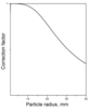
\begin{equation} \tag*{(8)} D=\frac{kT}{6\pi a\nu\rho_{air}}E(a), \end{equation}where $\nu$ is the kinematic viscosity of air, $\rho_{air}$ is the air density and $E(a)$ is the correction factor found by Phillips, 1975,
\begin{equation} \tag*{(9)} E(a)= \displaystyle {\frac{15+12c_1Kn+9(c_1^2+1)Kn^2+18c_2(c_1^2+2)Kn^3}{15-3c_1Kn+c_2(8+\pi\delta)(c_1^2+2)Kn^2}},\;\; \end{equation}with
\begin{eqnarray*} c_1=\frac{2-\delta}\delta, \qquad c_2=\frac1{2-\delta} \end{eqnarray*}and $\delta$ being a factor $<1$ entering a slip boundary conditions (Eq. (9)) of Phillips' paper. The Knudsen number $Kn=\lambda/a$ with $\lambda$ being the mean free path of the carrier gas molecules ($\lambda=65$ nm for air at ambient conditions). The parameter $\delta$ changes within 0.79 – 1. Equation (9) describes the transition correction for all Knudsen numbers and gives the correct limiting values (continuous and free-molecule ones). In what follows we put $\delta=1$.
|
| Figure 1 |
|
| Figure 2 |
We assume that
\begin{equation} \tag*{(10)} C(t)=\frac{C_0}{1+|A|}[1-A\cos(2\pi t/T)], \end{equation}where $T=24$ h, $C_0$ is a characteristic concentration of condensable vapors (a fitting parameter) and $-1< A\le1$. This function is maximal at midday. The concentration $C_0={\rm max}[C(t)]$ is a fitting parameter.
Next,
\begin{eqnarray*} v_T=\sqrt{\frac{8kT}{\pi m}}=0.906\cdot\,\rm10^4\,cm/s.,\quad V_0=3\cdot10^{-21}\,\rm cm^3, \end{eqnarray*} \begin{eqnarray*} \beta=0.6\cdot10^{-17}\,\rm cm^4/s. \end{eqnarray*}
We parametrize the particle source as $J=J(t)f(a)$, where
\begin{equation} \tag*{(11)} J(t)=J_0\left[\frac{1-B\cos(2\pi( t+\tau))/T)}{1+|B|}\right]^s. \end{equation}Again, $J_0$ is a fitting parameter and $-1 \gt B \le 1 $. The parameter $s$ is chosen between 3 and 10, the advance time $\tau$ varies between 0 and 12 h, i.e. it allows the source to act at nighttime. We will see that this parameter is of great importance.
The function $f$ is just a lognormal distribution,
\begin{equation} \tag*{(12)} f(a)da=\frac1{a\sqrt{2\pi}\ln\sigma}\exp\left[-\frac{(\ln(a/a_0))^2}{2(\ln\sigma)^2} \right]da. \end{equation}Here $a_0$ is a characteristic size of the particle forming by the nucleation source. The function $f$ is dimensional ($\rm cm^{-1}$).
The width of the distribution $\sigma$ varies within the interval [0.5 – 1.5].
Other parametrizations can be found in Kerminen et al., (2004a)
The continuity equation
\begin{equation} \tag*{(13)} \frac{\partial n}{\partial t}+\beta C\frac{\partial n}{\partial a}+\lambda n=J(a,t), \end{equation}can be solved exactly. Here $\beta=$const, $C=C(t)$, $\lambda=\lambda(a)$, i.e. we assume that the sizes of newly born particles are smaller than the molecular mean free path and the concentration of preexisting aerosol responsible for the sinks slowly changes with time. The details of the solution are given in Appendix B. The final result is (see also [Clement, 1978;, Williams and Loyalka, 1991])
\begin{eqnarray*} n(a,t)=\int_0^t J(a-\alpha(t,t'),t') e^{-\int_{t'}^t\lambda(a-\alpha(t,t"))dt"}dt'+ \end{eqnarray*} \begin{equation} \tag*{(14)} e^{-\int_0^t\lambda(a-\alpha(t,t'))dt'}n_0(a-\alpha(t,0)), \end{equation}where
\begin{equation} \tag*{(15)} \alpha(t,t')=\int_{t'}^t\beta C(t")dt". \end{equation}For $C(t)$ given by Eq. (10) one readily finds
\begin{equation} \tag*{(16)} \alpha(t,t')=a_g [g(2\pi t/T)-g(2\pi t'/T)], \end{equation}where
\begin{equation} \tag*{(17)} a^*=\frac{\beta C_0T}{2\pi(1+|A|)} \end{equation}and
\begin{equation} \tag*{(18)} g(x)=x-A\sin x. \end{equation}A new characteristic size $a^*$ (the growth parameter) appears, whose meaning is transparent: it is (approximately) the change to the particle size during the the whole growth period $T$. At $C_0=1$ ppt and $T=24$ h $a^*=23$ nm ($A=1$).
Next, the change to the total number concentration during this period is
\begin{equation} \tag*{(19)} n^*=\frac{J_0T}{2\pi(1+|B|)^s}. \end{equation}This result is the consequence of the source parametrization Eq. (11). It is seen that $n^*\approx1.2\cdot\rm10^4\,cm^{-3}$ at $J_0=1\,\rm cm^{-3}s^{-1}$ and $a^*=10$ nm at $C_0=10^7\,\rm cm^{-3}$.
The main result of this paper is the formulation of a simple model of atmospheric nucleation bursts. This model is analytically solvable and thus enormously simpler than the models currently used at present time. We have shown that the aerosol and chemical blocks can be considered independently. In principle, it is possible to use the data computed from the chemical block as the external parameters for this model. From this point of view all existing models are linear. Simply their authors did not notice the linearity of the aerosol growth process. Two exceptions are the works of Kerminen and Kulmala, [2002] and Lehtinen et al., [2007] who used the linear growth equation in the steady-state limit in order to link the concentration of just born particles with that of larger observable particles.
The main cause for the linearity is the preexisting aerosol whose concentration and size is enough for creating large coagulation sinks. The corresponding characteristic time is short compared to the time of self-coagulation. The particle production rate in the linear model is introduced as a fitting parameter. This step removes any traces of nonlinearity.
The fact that the particle formation-growth process is linear helps us to understand the mechanisms of the nucleation burst.
The spectrum $n(a,t)$ has the dimensionality $\rm cm^{-4}$. It is convenient to measure it in units of $n^*/a_0$, where the characteristic size $a_0$ of freshly formed particles is introduced in Eq. (12). We also notice that the function $a_0f(a)$ depends on the ratio $a/a_0$ (see Eq. (12)), which means that the particle size is measured in units of $a_0$. Next, it is convenient to measure $t$ in hours. It is essential to emphasize that the multiplier $n^*/a_0$ enters linearly into the expression for the particle spectrum Eq. (14), so all our plots operate with the ratio $n(a,t)a_0/n^*$.
The final size distribution is given by the analytical formula Eq. (14) which includes two dimensionless groups $a^*$ (the growth parameter) and $\lambda^*=\lambda T/2\pi$ (the sink parameter).
\begin{eqnarray*} a^*=\frac{\alpha C_0T}{2\pi b(1+|A|)}\qquad \lambda^*=\frac{\lambda T}{2\pi} \end{eqnarray*}The source rate $J_0$ enters the expression for the spectrum linearly and defines the characteristic concentration of freshly formed particles,
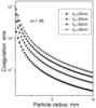
\begin{eqnarray*} n^*=\frac{J_0T}{2\pi(1+|B|)^s} \end{eqnarray*}There are also a couple of dimensionless parameters $A$ and $B$ defining the variability of the concentration of the condensing vapor and the source. Our numerical calculation were done for the sets
\begin{eqnarray*} & a^*=10,30,\quad\lambda^*=1,10,100,\quad A=0.5,\quad B=1, & & b=1nm,\quad s=6. & \end{eqnarray*}These parameters correspond to $C_0\approx10^7cm^{-3}$, $C_0\approx3\cdot10^7cm^{-3}$ and $\lambda=10^{-4}s^{-1}$, $\lambda=10^{-3}s^{-1}$, $\lambda=10^{-2}s^{-1}$ typical for the nucleation events observed in Hyytiälä [Dal Maso et al., 2005]. The source intensity enters as a multiplier to the expressions for the size spectra, so they are given in relative units (r.u.). For the same reason (linearity of the growth process) the average particle radius is independent of the particle source intensity $J_0$.
The linearity of the model means that the particle size distribution can be schematically presented as follows:
\begin{equation} \tag*{(20)} n(a,t)=\hat{\cal G}J+\hat{\cal F}n_0. \end{equation}Here $\hat{\cal G}$, $\hat{\cal F}$ are linear evolution operators allowing for restoring the full size distribution functions by the particle source $J$ and the initial conditions $n_0$. As we will see the first term does not produce a "burst-like" picture, although diurnal increases in the detectable particle concentration are well reproduced. The second term is of special significance. We show that if the source does not work at night time, but a highly disperse (undetectable) aerosol appears from somewhere, then a running-wave type picture typical for the nucleation burst arises. We incline to associate the nucleation events to this very mechanism. The overall situation is displayed in Figure 3. The initially existing fine undetectable aerosol begins to grow in parallel with the particles from the regular (periodic) source. The linearity of Eq. (1) is the reason for this running wave picture. Very likely that this initial aerosol (proto-aerosol in what follows) is closely related to stable clusters whose existence was theoretically predicted by Kulmala et al, [2000].
 |
| Figure 4 |
Figure 4 also shows an event picture. Although the daytime increase in the particle number concentration of the nucleation mode occurs, it is not so clearly expressed as in the case displayed in Figure 3.
 |
| Figure 5 |
A non-event picture is shown in Figure 5. Although the source produces the aerosol particles they do not overgrow the 3nm size and thus undetectable by existent standard spectroscopes.
 |
| Figure 6 |
Another type of nucleation burst is shown in Figure 6. If the source abruptly (at $t=t_c$) ceases to produce fresh particles then the particles produced before $t_c$ begin to grow in free regime and their spectrum moves to the right along the size axis as a running wave. There are some reasons to believe that such type of nucleation burst can realize in the atmosphere. The activity of the nucleation process can be suppressed by a slight increase in the concentration of preexisting particles [Lushnikov and Kulmala, 2000a; 2000b; 2004].
 |
| Figure 7 |
 |
| Figure 8 |
The last and very plausible scenario of the nucleation burst assumes that the source of nucleated particles $J$ works at nighttime (dark nucleation), whereas the condensable (but not nucleating) substances produced by photochemical processes appear only at daytime. This can happen, for example, if one of the participants of the cycle that results to nucleating substance is able to actively react with a product appeared in the photochemical cycle. In this case this product serves as an inhibitor of the nucleation process. If the total concentration of the aerosol particles accumulated during the dark time is not large (in order to exclude the coagulation growth) then these particles serve as the protoaerosol at the daytime. Our model allows us to calculate what is going on in this case. The calculations of Figure 7 are performed with the same parameter as in Figure 8, but the maximum of the source was shifted by 12h earlier. Figure 7 displays the results. Instead of rather smooth development of events (see Figure 7) a narrow peak moving to the right appears. This scenario well reproduces the picture of the "heterogeneous" nucleation burst, where the nucleated particles and their coating have different origination.
In this paper we have considered the possibility to apply a linear evolution model for describing the nucleation bursts observed in boreal forests. The simplifications introduced by us rely upon the fact that the evolution of chemical content of the atmosphere is entirely determined by condensational sinks, where the contribution of accumulation mode is overwhelming as compared to that of the nucleation mode. This statement means that the newly born particles does not affect the chemical kinetics of the trace gases responsible for production of low volatile substances giving then rise the life to the aerosol particles. The chemical block of any model describing the formation of disperse phase in the atmosphere can be considered independently of the block describing the particle formation, growth, and death. It is not yet enough for reaching the linearity of the particle growth model. The nucleation and coagulation are essential sources of nonlinearity. We have thus sacrificed the self-coagulation of the particles of the nucleation mode whereas the intermode coagulation is replaced by the coagulation sinks which are formed by the particles of the accumulation mode. This approximation is also well grounded under the condition, where the self-coagulation time is much longer than the time of intermode coagulation.
Much more risky is our replacement of the nucleation by an external particle source whose productivity has been introduced as a fitting parameter. On the other hand, we know almost nothing about the kinetics of the nucleation process as well as its participants. Moreover, at sufficiently high nucleation rates coagulation of newly born particles can complicate the process.
And at last, we introduced the growth rate which was considered to be independent of the particle size. We thus sacrificed the dependence due to Kelvin's effect because of our very poor knowledge of the physico-chemical properties of small particles.
We thus have come to the linear model of the particle formation-growth, i.e., the evolution equation governing the particle size distribution reduced to the linear one. This is the main and very principle difference of our model from other ones.
Although our model comparatively primitive it has many advantages. They are:
The dynamics of particle formation growth strongly depends on the initial conditions. There are three possibility:
And, at last, the source produces fresh particles, but we do not see them because their growth is suppressed with strong condensation and coagulation sinks. The particles of the nucleation mode do not overstep the detectable size 3 nm.
The coagulation sink $\lambda$ is either a fitting parameter or can be calculated if we know $N(b,t)$, the size distribution of the preexisting particles
\begin{equation} \tag*{(A.1)} \lambda(a)=\int K(a,b)N(b,t) db, \end{equation}where $K(a,b)$ is the coagulation efficiency. In contrast to commonly accepted recipes we calculate the specific coagulation sink, i.e., the sink for the concentration $N=1\,cm^{-3}$.
In what follows we assume that $N(b)$ is described by a lognormal function
\begin{equation} \tag*{(A.2)} f(a)da=\frac1{a\sqrt{2\pi \sigma}}\exp\left[-\frac1{2\sigma}\ln^2(a/b_0)) \right]d a \end{equation}Here $b_0$ is a characteristic size of the preexisting mode. The function $f$ is dimensional ($\rm cm^{-4}$).
The coagulation efficiencies are assumed to be,
\begin{equation} \tag*{(A.3)} K(a,b)=\frac{2\pi(a+b)^2v_T(a,b)}{1+\sqrt{1+\displaystyle{\left(\frac{(a+b)v_T(a,b)}{2D(a,b)}\right)^2}}} \end{equation}Here $a,b$ are the radii of the colliding particles,
\begin{eqnarray*} v_T(a,b)=\sqrt{\frac{8kT}{\pi\mu_{a,b}}} \end{eqnarray*}is the thermal velocity,
\begin{equation} \tag*{(A.4)} \mu_{a,b}=\frac{m_am_b}{m_a+m_b} \end{equation}is the reduced mass, with $m_a,\, m_b$ being the masses of colliding particles,
\begin{equation} \tag*{(A.5)} D_{a,b}=D_a+D_b \end{equation}is the diffusivity of the colliding pair, $D_a,\,D_b$ are the diffusivity of each particle (should be found for the transition regime),
\begin{equation} \tag*{(A.6)} D=\frac{kT}{6\pi a\nu\rho_{air}}C(a) \end{equation}where $\nu$ is the kinematic viscosity of air, $\rho_{air}$ is the air density and $C(a)$ is given by the formula that can be used instead of the Millikan correction, [Phillips, 1975]
\begin{equation} \tag*{(A.7)} C(a)=\frac{15+12c_1Kn+9(c_1^2+1)Kn^2+18c_2(c_1^2+2)Kn^3}{15-3c_1Kn+c_2(8+\pi\delta)(c_1^2+2)Kn^2} \end{equation}where
\begin{eqnarray*} c_1=\frac{2-\delta}\delta, \qquad c_2=\frac1{2-\delta} \end{eqnarray*}with $\delta$ being a factor $<1$ entering the slip boundary condition [Phillips, 1975]. The Knudsen number $Kn=\lambda/a$ with $\lambda$ being the mean free path of the carrier gas molecules. The parameter $\delta$ changes within $0.79$ – $1$. (see the paper). We use the density of aerosol particles $\rho=2$ g$\cdot$cm$^{-3}$ and $\delta=1$
Technically it is more convenient to have the result presented in the form
\begin{equation} \tag*{(A.8)} \lambda(a,b)=\Lambda(l)f(\tilde a,\tilde b) \end{equation}where $l$ is a scale and $\tilde a=a/l$, $\tilde b=b/l$. The value of this scale depends on our good will. We choose $l=1\,\rm nm=10^{-7}\,cm$. Then all sizes in Eq. (A.8) are measured in nm. We have,
\begin{equation} \tag*{(A.9)} v_T(l)=\sqrt{\frac{8kT}{\pi\cdot(4\pi l^3/3)\rho}}, \end{equation}Then $\Lambda(l)$ in Eq. (A.8) is
\begin{equation} \tag*{(A.10)} \Lambda(l)=2\pi\sqrt{\frac{6kTl}{\pi^2\rho}}=2.23\cdot10^{-10}s^{-1}, \end{equation}and the numerator of $K$ in Eq. (A.3) takes the form:
\begin{equation} \tag*{(A.11)} 2.23\cdot10^{-10}(\tilde a+\tilde b)^2\sqrt{\frac{\tilde a^3+\tilde b^3}{\tilde a^3\tilde b^3}} \end{equation}The same combination appears in the denominator of Eq. (A.3). We thus find,
\begin{equation} \tag*{(A.12)} \left(\frac{(a+b)v_T(a,b)}{2D(a,b)}\right)^2=0.0147\left(\frac{\tilde a+\tilde b}{\tilde b C(\tilde a)+\tilde a C(\tilde b)} \sqrt{\frac{\tilde a^3+\tilde b^3}{\tilde a\tilde b}} \right)^2. \end{equation}The mean free path in the expression for $C$ is taken 60 nm, $T=300$K. We have $K(\tilde a,\tilde b)=\Lambda F(\tilde a,\tilde b)$, where
\begin{equation} \tag*{(A.13)} F(\tilde a,\tilde b)=\frac{(\tilde a+\tilde b)^2\displaystyle{\sqrt{\frac{\tilde a^3+\tilde b^3}{\tilde a^3\tilde b^3}}}}{1+{\displaystyle \sqrt{1+0.0147\left[\frac{\tilde a+\tilde b} {\tilde b C(\tilde a)+\tilde a C(\tilde b)}\sqrt{\frac{\tilde a^3+\tilde b^3}{\tilde a\tilde b}} \right]^2}}} \end{equation}Finally, the specific coagulation sink is expressed as follows:
\begin{equation} \tag*{(A.14)} \lambda(\tilde a)=\frac{2.23\cdot10^{-10}}{\sqrt{2\pi \sigma}} \int\limits_0^\infty\exp\left[-\frac1{2\sigma}\ln^2(\tilde b/\tilde b_0)) \right]F(\tilde a,\tilde b)\frac{d \tilde b}{\tilde b} \end{equation}The scale of the lognormal distribution $\tilde b_0$ is measured in nm and $\lambda$ in ${\rm cm^3\cdot s^{-1}}$
In this appendix we solve the continuity equation. This solution appeared many times in the scientific literature (see [Clement, 1978; Williams and Loyalka, 1991]. Here we reproduce the solution of (B.1) in more detail that this was done earlier.
We look for the solution to the equation for the function $n(a,t)$
\begin{equation} \tag*{(B.1)} \frac{\partial n}{\partial t}+\beta C\frac{\partial n}{\partial a}+\lambda(a,t) n=J(a,t), \end{equation}assuming that the initial particle spectrum $n(a,0)=n_0(a)$ is a known function. Here $\beta=$const, $C=C(t)$, i.e., we assume that the sizes of newly born particles is smaller than the molecular mean free path. The functions $J(a,t)\ge0$ and $\lambda(a,t)\ge0$ are defined only for positive $a$. At $a<0$ both these functions are equal to zero.
We look for $n(a,t)$ as the solution to the equation
\begin{equation} \tag*{(B.2)} R(n,a,t)=0 \end{equation}with respect to $n$. The equation for $R$ readily follows from Eq. (B.1). Indeed, the derivatives of $n$ with respect to $t$ and $a$ are expressed in terms of $R$ as follows: $n'_t=-(R'_t)/(R'_n)$ and $n'_a=-(R'_a)/(R'_n)$. Here prime stands for partial differentiation over the argument shown in the superscript. On substituting this into Eq. (B.1) gives the partial differential equation for $R=R(n,a,t)$
\begin{equation} \tag*{(B.3)} \frac{\partial R}{\partial t}+\beta C\frac{\partial R}{\partial a}+(J-\lambda n)\frac{\partial R}{\partial n}=0. \end{equation}The equations for the characteristics of Eq. (B.3) are:
\begin{equation} \tag*{(B.4)} \frac{dt}{1}=\frac{da}{\beta C}=\frac{dn}{J(a,t)-\lambda(a,t)n}. \end{equation}This is the set of two ordinary differential equations for $n(t)$ and $a(t)$. The first characteristics is readily found from the first equation of the set (B.4),
\begin{equation} \tag*{(B.5)} a(t)=a_c+\alpha(t), \end{equation}where $a_c$ is the integration constant and $\alpha(t)=\beta\int_0^tC(t')dt'$.
The second one is found from the second equation of this set,
\begin{equation} \tag*{(B.6)} \frac{dn}{dt}+\lambda(a(t),t) n=J(a(t),t), \end{equation}where $a(t)$ is given by Eq. (B.5). Then one finds,
\begin{equation} \tag*{(B.7)} !n(t)=[n_c+\int_0^t J(a_c+\alpha(t'),t')e^{\int_0^{t'}\lambda(a_c+\alpha(t"), t")dt"}dt'] \times e^{-\int_0^t\lambda(a_c+\alpha(t'),t')dt'}, \end{equation}Here $n_c$ is the integration constant of Eq. (B.6).
Now we introduce two functions,
\begin{eqnarray*} a_c(a,t)=a-\alpha(t)\qquad \rm and \end{eqnarray*} \begin{equation} \tag*{(B.8)} n_c(n,a,t)=ne^{\int_0^t\lambda(a_c(a,t)+\alpha(t'),t')dt'}- \int_0^t J(a_c(a,t)+\alpha(t'),t')e^{\int_0^{t'}\lambda(a_c(a,t)+\alpha(t"),t")dt"}dt'. \end{equation}Equations (B.5) and (B.6) allow us to conclude that the function
\begin{equation} \tag*{(B.9)} R(n,a,t)=R(n_c(n,a,t), a_c(a,t)) \end{equation}is the solution to Eq. (B.3).
On solving then Eq. (B.9) with respect to $n(a,t)$ yields
\begin{equation} \tag*{(B.10)} n(a,t)= \int_0^t J(a-\alpha(t)+\alpha(t'),t')e^{-\int_{t'}^t\lambda(a-\alpha(t)+\alpha(t"),t")dt")}dt'+ e^{-\int_0^t\lambda(a-\alpha(t)+\alpha(t'),t')dt'}n_0(a-\alpha(t))& \end{equation}where the function $n_0(x)$ should be determined from the initial conditions. For the separable source and zero initial conditions we have,
\begin{eqnarray*} n(a,t)= \end{eqnarray*} \begin{equation} \tag*{(B.11)} \!\!\!\!\int_0^t f[a-\alpha(t)+\alpha(t')]J(t')e^{-\int_{t'}^t\lambda(a-\alpha(t)+\alpha(t"),t")dt"}dt'. \end{equation}Next,
\begin{equation} \tag*{(B.12)} \alpha(t)=\frac{\beta C_0}{1+|A|}[1-A\cos(2\pi t/T)] \end{equation} \begin{eqnarray*} \!\!\!\!\!\!\!\!\!\!\!\!\!\!\!\!{\rm or} \quad\quad\quad\quad \frac{\beta C_0}{1+|A|}\int_{t'}^t\frac12(1+\sin(2\pi t"/T))dt"= \end{eqnarray*} \begin{equation} \tag*{(B.13)} \frac{\beta C_0T}{2\pi(1+|A|)} [g(2\pi t/T)-g(2\pi t'/T)] \end{equation}where
\begin{equation} \tag*{(B.14)} g(x)=x-A\sin x \end{equation}Aalto, P., et al. (2001), Physical characterization of aerosol particles during nucleation events, Tellus, 53B, p. 344–358, doi:10.3402/tellusb.v53i4.17127.
Adams, P. J., J. H. Seinfeld (2002), Predicting global aerosol size distribution in general circulation models, J. Geophys. Res., 107, no. D19, p. 4370, doi:10.1029/2001JD001010.
Adams, P. J., J. H. Seinfeld (2003), Disproportionate impact of particulate emissions on global cloud condensation nuclei concentration, Geophys. Res. Lett., 30, p. 1239, doi:10.1029/2002GL016303.
Anttila, T., V.-M. Kerminen, M. Kulmala, A. Laaksonen, C. D. O'Dowd (2004), Modelling the formation of organic particles in the atmosphere, Atmos. Chem. Phys., 4, p. 1071–1083, doi:10.5194/acp-4-1071-2004.
Barrett, J. C., C. F. Clement (1991), Aerosol concentrations from a burst of nucleation, J. Aerosol Sci., 22, p. 327–335, doi:10.1016/S0021-8502(05)80010-2.
Boy, M., M. Kulmala (2002), Nucleation events on the continental boundary layer: in uence of physical and meteorological parameters, Atmos. Chem. Phys., 2, p. 1–16, doi:10.5194/acp-2-1-2002.
Boy, M., U. Rannik, K. E. Lehtinen, V. Tarvainen, H. Hakola, M. Kulmala (2003), Nucleation events in the continental boundary layer: Long-term statistical analysis of aerosol relevant characteristics, J. Geophys. Res., 108, no. D21, p. 4667–4675, doi:10.1029/2003JD003838.
Clement, C. F. (1978), Solutions of the continuity equation, Proc. R. Soc., London, A364, p. 117–119.
Clement, C. F., I. J. Ford (1999), Gas to particle conversion in the atmosphere: II Analytic models of nucleation bursts, Atmos. Environment, 33, p. 489–499, doi:10.1016/S1352-2310(98)00265-9.
Clement, C. F., L. Pirjola, C. H. Twohy, I. J. Ford, M. Kulmala (2006), Analytic and numerical calculations of the formation of a sulfuric acid aerosol in the upper troposphere, J. Aerosol Sci., 37, p. 1717–1729, doi:10.1016/j.jaerosci.2006.06.007.
Dal Maso, M., M. Kulmala, K. E. J. Lehtinen, J. M. Mäkelä, P. Aalto, C. D. O'Dowd (2002), Condensation and coagulation sinks and formation of nucleation mode particles in coastal and boreal boundary layers, J. Geophys. Res., 107, p. D19, doi:10.1029/2001JD001053.
Dal Maso, M., M. Kulmala, I. Riippinen, T. Hussein, R. Wagner, P. P. Aalto, K. E. J. Lehtinen (2005), Formation and Growth of fresh Atmospheric Aerosols: Eight Years of Aerosol Size Distribution Data from SMEAR II, Hyytiälä, Finland, Boreal Env. Res., 10, p. 323–336.
Easter, R. C., et al. (2004), MIRAGE: Model description and evaluation of aerosols and trace gases, J. Geophys. Res., 109, p. D20210, doi:10.1029/2004JD004571.
Elperin, T., A. Fominykh, B. Krasovitov, A. Lushnikov (2013), Isothermal absorption of soluble gases by atmospheric nanoaerosols, Phys. Rev., E87, p. 012807, doi:10.1103/PhysRevE.87.012807.
Friedlander, S. K. (1977), Smokes, Dust and Haze, Wiley, New York.
Friedlander, S. K. (1983), Dynamics of Aerosol Formation by Chemical Reactions, 354–363 pp., Ann. NY Acad. Sci., NY.
Griffin, R., D. R. Cocker III, R. Flagan, J. H. Seinfeld (1999), Organic aerosol formation from the oxidation of biogenic hydrocarbons, J. Geophys. Res., 104, p. 3555–3567, doi:10.1029/1998JD100049.
Griffin, R., D. Dabdub, J. H. Seinfeld (2002), Secondary organic aerosol I. Atmospherical chemical mechanism for production of molecular constituents, J. Geophys. Res., 107, no. D17, p. 4332, doi:10.1029/2001JD000541.
Grini, A., H. Korhonen, K. Lehtinen, I. Isaksen, M. Kulmala (2005), A combined photochemistry/aerosol dynamics model: model development and a study of new particle formation, Boreal Environ. Res., 10, p. 525–541.
Hoffmann, Th., J. Odum, F. Bowman, D. Collins, D. Klockow, R. C. Flagan, J. H. Seinfeld (1997), Formation of organic aerosols from the oxidation of biogenic hydrocar-bons, J. Atmos. Chem., 26, p. 189–222, doi:10.1023/A:1005734301837.
Janson, R., K. Rozman, A. Karlsson, H. C. Hansson (2001), Biogenic emission and gaseous precursor to forest aerosols, Tellus, 53B, p. 423–440, doi:10.3402/tellusb.v53i4.16615.
Kavouras, I. G., N. Mihalopoulos, E. G. Stephanou (1998), Formation of atmospheric particles from organic acids produced by forests, Nature, 395, p. 683–686, doi:10.1038/27179.
Kerminen, V.-M., M. Kulmala (2002), Analytical formulae connecting the "real" and the "apparent" nucleation rate and the nuclei number concentration for atmospheric nucleation events, J. Aerosol Sci., 33, p. 609–622, doi:10.1016/S0021-8502(01)00194-X.
Kerminen, V.-M., T. Anttila, K. E. J. Lehtinen, M. Kulmala (2004a), Parametrization for atmospheric new-particle formation: application to a system involving sulfuric acid and condensable water-soluble organic vapors, Aerosol Sci. Technol., 38, p. 1001–1008, doi:10.1080/027868290519085.
Kerminen, V.-M., K. Lehtinen, T. Anttila, M. Kulmala (2004b), Dynamics of atmospheric nucleation mode particles: timescale analysis, Tellus, B56, p. 135–146, doi:10.3402/tellusb.v56i2.16411.
Kerminen, V.-M., L. Pirjola, M. Kulmala (2001), How signi cantly does coagulation scavenging limit atmospheric particle production?, J. Geophys. Res., 106, no. D20, p. 24,119–24,125, doi:10.1029/2001JD000322.
Kerminen, V.-M., A. Virkkula, R. Hillamo, A. S. Wexler, M. Kulmala (2000), Secondary organics and atmospheric cloud condensation nuclei production, J. Geophys. Res., 105, p. 9255–9264, doi:10.1029/1999JD901203.
Korhonen, H., K. E. J. Lehtinen, L. Pirjola, I. Napari, H. Vehkamaki, M. Noppel, M. Kulmala (2003), Simulation of atmospheric nucleation mode: a comparison of nucleation models and size distribution representations, J. Geophys. Res., 108, p. D15, doi:10.1029/2002JD003305.
Korhonen, H., K. E. J. Lehtinen, M. Kulmala (2004), Multicomponent aerosol dynamic model UHMA: Model development and validation, Atmos. Chem. Phys. Discuss., 4, p. 471–506, doi:10.5194/acpd-4-471-2004.
Kulmala, M. (2003), How particles nucleate and grow, Science, 302, p. 1000–1001, doi:10.1126/science.1090848.
Kulmala, M., H. Tammet (2007), Finnish-Estonian air ion and aerosol workshop, Boreal Env. Res., 12, p. 237–245.
Kulmala, M., M. Dal Maso, J. Mäkelä, L. Pirjola, M. Väkeva, P. Aalto, P. Miikkulainen, K. Hämmeri, C. O'Dowd (2001), On the formation, growth and composition of nucleation mode particles, Tellus, B53, p. 479–490, doi:10.3402/tellusb.v53i4.16622.
Kulmala, M., P. Hari, A. Laaksonen, Y. Viisanen (2005), Research unit of physics, chemistry and biology of atmospheric composition and climate change: overview of recent results, Boreal Env. Res., 10, p. 459–478.
Kulmala, M., V.-M. Kerminen, A. Laaksonen (1995), Simulation on the effect of sulfuric acid formation on atmospheric aerosol concentration, Atmos. Environ., 29, p. 377–382, doi:10.1016/1352-2310(94)00255-J.
Kulmala, M., H. Vehkmäki, T. Petäjä, M. Dal Maso, A. Lauri, V.-M. Kerminen, W. Birmili, P. H. McMurry (2004a), Formation and growth rates of ultrafine atmospheric particles: a review of observations, J. Aerosol Sci., 35, p. 143–176, doi:10.1016/j.jaerosci.2003.10.003.
Kulmala, M., V.-M. Kerminen, T. Anttila, A. Laaksonen, C. D. O'Dowd (2004b), Organic aerosol formation via sulfate cluster activation, J. Geophys. Res., 109, no. D4, p. 4205, doi:10.1029/2003JD003961.
Kulmala, M., L. Laakso, K. E. J. Lehtinen, I. Riipinen, M. Dal Maso, T. Anttila, V.-M. Kerminen, U. Horrak (2004c), Initial steps of aerosol growth, Atmos. Chem. Phys., 4, p. 2553–2560, doi:10.5194/acp-4-2553-2004.
Kulmala, M., K. E. J. Lehtinen, A. Laaksonen (2006), Cluster activation theory as an explanation of the linear dependence between formation rate of 3 nm particles and sulphuric acid concentration, Atmos. Chem. Phys., 6, p. 787–793, doi:10.5194/acp-6-787-2006.
Kulmala, M., L. Pirjola, J. M. Mäkelä (2000), Stable sulfate clusters as a source of new atmospheric particles, Nature, 404, p. 66–69, doi:10.1038/35003550.
Kulmala, M., et al. (2007), The condensation particle counter battery (CPCB): A new tool to investigate the activation properties of nanoparticles, J. Aerosol Sci., 38, p. 289–304, doi:10.1016/j.jaerosci.2006.11.008.
Lehtinen, K. E. J., M. Kulmala (2003), A model for particle formation and growth in the atmosphere with molecular resolution in size, Atmos. Chem. Phys., 3, p. 251–257, doi:10.5194/acp-3-251-2003.
Lehtinen, K. E. J., M. Dal Maso, M. Kulmala, V.-M. Kerminen (2007), Estimating nucleation rates from apparent particle formation rates and vice-versa: revised formulation of the Kerminen-Kulmala equation, J. Aerosol Sci., 38, p. 988–994, doi:10.1016/j.jaerosci.2007.06.009.
Lushnikov, A. A., M. Kulmala (2000a), Foreign aerosol in nucleating vapor, J. Aerosol Sci., 31, p. 651–672, doi:10.1016/S0021-8502(99)00553-4.
Lushnikov, A. A., M. Kulmala (2000b), Nucleation burst in a coagulating system, Phys. Rev., E62, p. 4932–4939, doi:10.1103/PhysRevE.62.4932.
Lushnikov, A. A., M. Kulmala (2004), Flux-matching theory of particle charging, Phys. Rev., E70, p. 046413(1–9).
Lushnikov, A. A., A. D. Gvishiani, Yu. S. Lyubovtseva (2013a), Trapping of trace gases by atmospheric aerosols, Russ. J. Earth Sci., 13, p. ES2002, doi:10.2205/2013ES000530.
Lushnikov, A. A., A. D. Gvishiani, Yu. S. Lyubovtseva (2013b), Fractals in the atmosphere, Russ. J. Earth Sci., 13, p. ES2002, doi:10.2205/2013ES000531.
Lushnikov, A. A., V. A. Zagaynov, Yu. S. Lyubovtseva, A. D. Gvishiani (2014), Nanoaerosol formation in the troposphere under action of cosmic radiation, Atmospheric and Oceanic Physics, 50, no. 2, p. 152–159, doi:10.1134/S0001433814020078.
Lyubovtseva, Yu. S., L. Sogacheva, M. Dal Maso, B. Bonn, P. Keronen, M. Kulmala (2005), Seasonal variations of trace gases, meteorological parameters, and formation of aerosols in boreal forests, Boreal Environ. Res., 10, p. 493–510.
O'Dowd, C., P. Aalto, K. Hämeri, M. Kulmala, T. Hoffmann (2002), Aerosol formation: atmospheric particles from organic vapors, Nature, 416, p. 497–498, doi:10.1038/416497a.
Phillips, W. F. (1975), Drag on a small sphere moving through a gas, Phys. Fluids, 18, p. 1089–1093, doi:10.1063/1.861292.
Spracklen, D. V., K. S. Carslaw, M. Kulmala, V.-M. Kerminen, G. V. Mann, S.-L. Sihto (2006), The contribution of boundary layer nucleation events to total particle concentration on regional and global scales, Atmos. Chem. Phys., 6, p. 5631–5648, doi:10.5194/acp-6-5631-2006.
Stolzenburg, M. R., P. H. McMurry, H. Sakurai, J. N. Smith, R. L. Mauldin, F. L. Eisele, C. F. Clement (2005), Growth rates of freshly nucleated atmospheric particles in Atlanta, J. Geophys. Res., 110, no. D22, p. D22S05, doi:10.1029/2005JD005935.
Williams, M. M. R., S. K. Loyalka (1991), Aerosol Science, Theory and Practice, Pergamon Press, Oxford, New York, Seoul, Tokyo.
Zhang, Y., C. Seigneur, J. H. Seinfeld, M. Z. Jacobson, F. S. Binkowski (1999), Simulation of aerosol dynamics: A comparative review of algorithms in air quality models, Aerosol Sci. Technol., 31, p. 487–514, doi:10.1080/027868299304039.
Received 8 October 2017; accepted 26 October 2017; published 2 November 2017.

Citation: Lushnikov A. A., V. A. Zagaynov, Yu. S. Lyubovtseva (2017), Formation of aerosols in the lower troposphere, Russ. J. Earth Sci., 17, ES4001, doi:10.2205/2017ES000604.
Copyright 2017 by the Geophysical Center RAS.