3. Method for Observing Electric Fields and Neutral Winds With Backscatter From Field-Aligned Irregularities (FAI)

[34]  Most coherent scatter radars (CSRs) are operated at a frequency close to 50 MHz and observe perpendicularly to the geomagnetic field in the meridional plane. The backscatter signal is very aspect sensitive and disappears when the radar beam deviates by about 0.5^o from perpendicularity. Since 3-m irregularities cannot be generated directly, the line-of-sight Doppler velocity observed in the meridional plane is the line-of-sight phase velocity of the secondary waves. The beauty is that, independently of complexity and nonlinearity of the processes resulting in 3-m irregularities, their phase velocity is described to leading order by the same expression (equation (12)).

3.1. Identities of the Contributors to the Phase Velocity in the shape E Region

[35]  The obvious problem which one will face here is that from the measurements of only one parameter, namely the line-of-sight Doppler velocity, we are going to find several unknown ionospheric parameters: zonal and meridional electric fields and neutral winds. So, to succeed we obviously need some additional information and assumptions. Below we demonstrate the basis of the method for the routine observational geometry when the radar observes in the meridional plane. 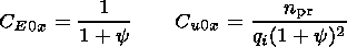Assuming that the line-of-sight Doppler velocity is the phase velocity of the secondary gradient drift waves, the phase velocity of secondary waves is described by (12).

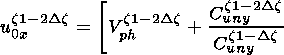
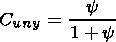
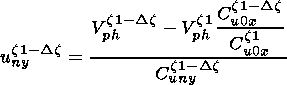
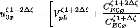
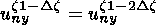
[36]  Equation (12) contains 4 unknown energy sources: a background zonal electric field, a zonal polarization electric field written in terms of the current velocity u_0x, meridional and zonal neutral winds. The relative plasma density fluctuation of the primary wave in equation (12) is not known either, although a reasonably good guess can be made based on evidence and simulation. We will discuss this point in more detail below. 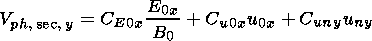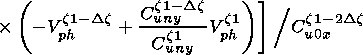We use the term background for the zero-order electric field meaning that its typical scale length is much larger than the typical scale of the polarization electric field produced by the primary waves.

[37]  Let us have a detailed look at the right-hand side (RHS) of equation (12). The zonal neutral wind in the last term in the braces has the coefficient compared to the meridional wind. For the lower E region q_i 1 and the contribution from the zonal wind can be neglected compared to that from the meridional wind. For the higher E region ions become magnetized and q_i >1, or even 1. In this case the zonal wind will dominate in the third term in equation (12), but the coefficient of the whole term becomes very small: y / q_i 1. Even for q_i =1, which for the MU radar corresponds to the altitudes 130-135 km, y 10^-4. Obviously, at these altitudes there does not exist a neutral wind capable of contributing noticeably to the phase velocity. Thus this term noticeably contributes to the phase velocity only in the lower E region by means of the meridional neutral wind. Above about 102 km the neutral wind does not affect the phase velocity.

Figure 2

[38]  Note also the polarization electric field (the second term in braces on RHS) decreases with increasing ion magnetization (increasing height) and the large-scale electric field defines the phase velocity above 120 km altitude. The abovementioned peculiarities are seen in Figure 2, in which we have plotted the coefficients of each of the three RHS terms in equation (12).

[39]  Going down in altitude q_i decreases. Below approximately 94-96 km this results in y >1 and the second and third terms in braces dominate the line-of-sight phase velocity. It can be seen also from Figure 2 where below 94 km the contribution from the background electric field becomes negligible. Thus the line-of-sight phase velocity at almost any altitude in the E region is defined by only two contributors.

[40]  The major part of E -region backscatter has been observed below 125 km. For the lower E region we may assume q_i <1 (which implies q_i² 1 and so allows us to neglect q_i² in comparison with 1) and rewrite (1) as

(18)

where

(19)

[41]  Now the left-hand side (LHS) of (18) is the measured line-of-sight Doppler velocity, and the right-hand side of (18) is a sum of contributions to the secondary gradient drift instability (GDI) written in terms of velocity. From left to right these contributors are: a large-scale "background" electric field (large scale in the sense that its typical scale length is much more than the typical scale length of the polarization electric field caused by the primary waves), a polarization electric field due to primary waves, and a line-of-sight neutral wind. Note that all three contributions to the RHS of equation (18) are unknown although at almost any altitude in the E region (as we have shown) only two of them define the line-of-sight phase velocity.

[42]  Note that the coefficients C_j are functions of local time, place and altitude and may be calculated for the time and location of each observational data set.

[43]  In Figure 2 we plot the dimensionless coefficients C_j of each contribution (the RHS terms in equations (12) and (18)) to the phase velocity (the LHS term in equation (18)) as a function of altitude for the general case of arbitrary ion magnetization. The phase velocity has the coefficient C_Vph =1. In calculating C_u0x we have assumed n pr = 5%. We explain our reasons for this assumption in the end of section 3.2.2. From Figure 2 it can clearly be seen that all coefficients C_j change rapidly with altitude due to the exponential altitude dependence of the collisional frequencies, but each exhibits a very different altitude behavior.

[44]  In Figure 2 the magnitudes of the electron and ion collisional frequencies in C_j were calculated using the formulas by Schunk and Nagy [2000]. The neutral densities and electron/ion temperature in the formulas for collisional frequencies ( T_e=T_i=T_n for the altitudes of interest) were calculated using the MSIS E 90 model [Hedin, 1991]. All quantities were calculated for the MU radar experiment on 1 October 2001 (Shigaraki, Japan, 34.9^oN, 136.1^oE) for the time 1000 LT. The gyrofrequencies were calculated in accordance with the geomagnetic field data from the IGRF model. Both models (MSIS E 90 and IGRF) may also be found on the National Space Satellite Data Center Web site http://nssdc.gsfc.nasa.gov/space/model/.

[45]  From Figure 2 it follows that for this given time and location: (1) the polarization electric field due to primary waves by itself defines the phase velocity near 98-102 km altitude ( C_u0x C_u0y, C_E0x ); (2) at altitudes of 90-94 km the contribution from the background electric field is negligible compared to that of neutral winds and the polarization electric field; and (3) above about 115 km the background electric field dominates the phase velocity. It can be seen that C_E0x decreases with altitude starting from 120 km, since the ions become more and more magnetized (the ion-neutral collisional frequency drops exponentially with altitude) and drift together with the electrons in crossed E B when w_i n_in.

3.2. Basis of the Method

3.2.1. Boundary condition.

[46]  Next we are going to apply our preliminary knowledge of the E -region processes. In accordance with E -region backscatter observations our principal interest is in the altitude range 90-120 km. Larsen [2002] has catalogued and analyzed over 400 neutral wind profiles collected since 1958. He has shown that at middle and low latitudes the wind velocity is maximum in the altitude range between l00 and 110 km and the maximum wind velocity has exceeded l00 m s^-1 in 60% of the observations. The maximum speed ever observed was between 160 and 170 m s^-1. On the basis of Larsen's [2002] analysis of wind data one may postulate u_n 170 m s^-1.

[47]  On the basis of the fact that the coefficients in equation (18) have very different altitude dependences (Figure 2) we will use the C_j as filters in the following. Let us suppose for a moment that only one of the contributions in the RHS of equation (18) defines the phase velocity (LHS of equation (18)) and calculate from the Doppler data and equations (18) and (19) what this phase velocity for each separate contributor would be if this were the case. To this end we calculate C_j in accordance with the scheme described above for the time and location corresponding to the time and location of each set of the Doppler measurements analyzed.

Figure 3

[48]  We plot C_j in Figure 3a and the observed phase velocity, the meridional neutral wind, and the zonal large-scale and polarization electric fields for this hypothesized case in Figure 3b for the MU radar observations at the time 0250:05.9 LT on 25 July 2001. In Figure 3b we show these supposed velocities as thin lines and mark in gray the area (confined by the dashed white lines) to indicate the observable velocity range 170 m s^-1. These white dashed lines show the maximum possible amplitude of wind velocities which have ever been observed in connection with type 2 backscatter at E -region equatorial and middle latitudes [Larsen, 2002].

[49]  From Figure 3 we see that there are altitude ranges where the filter velocities have magnitudes which have never been observed. This fact allows us to discard at some definite altitude those contributions whose velocity significantly exceeds 170 m s^-1 (the white dashed line in Figure 3). In doing so we use the coefficients C_j as filters which allow us to find the altitude(s) at which only one contributor defines the phase velocity. For the data in Figure 3 it is the polarization electric field near 99 km altitude. Thus we have found the boundary condition for the driving forces of the instability. The procedure has been repeated for each altitude profile of the phase velocity of the secondary waves.

[50]  The boundary condition is the basic starting point of our method. As a rule for almost any backscatter event in the E region at least one boundary condition exists. Near 100 km altitude it is as a rule for the polarization electric field as in the example discussed above. Above about 116 km the boundary condition is for the large-scale electric field. Near 94 km and below it is for the neutral wind.

[51]  Note, that the boundary condition is absolutely essential for the following procedure if we do not know the magnitude of any of the contributors to the line-of-sight phase velocity from measurements. In cases when one of these contributors is known (e.g., the large-scale electric field measured in the F region and mapping down to the E region) this fact can be used as a boundary condition (in our example for the altitudes above 100 km).

3.2.2. Reconstruction of winds and electric fields.

[52]  In the following we are going to use the boundary condition for reconstruction of neutral winds and electric fields. For each backscatter observation time (for the MU radar the time resolution may be as small as several seconds), we have a data set of Doppler velocities from the backscatter altitudes with an altitude step D z (the altitude resolution of the radar) and the boundary condition at the altitude z 1. We assume that the altitude resolution of the radar is good enough to consider the energy sources (neutral winds and electric fields) to be the same for two neighboring altitudes of observation. This assumption defines the resolution of our method and one has to decide if this altitude/time resolution is acceptable for his or her purposes.

[53]  In the following we demonstrate the data processing procedure for the case when we have the boundary condition at the altitude z 1 (99 km for the data set in Figure 3b) for the zonal polarization electric field written in terms of the current velocity u_0x^{z 1} (equation (18)). We then go step-by-step down (up) in altitude assuming that at the neighboring altitude z 1 - D z (z 1 + D z ) the current velocity remains the same: u_0x^{z 1} = u_0x^{z 1 - D z}.

[54]  As we have discussed above, from Figure 2 it follows that, as a rule, at any given altitude the phase velocity is defined by no more than two contributors. This gives us two equations for phase velocities (in the following we omit subindices sec, y ), V_ph^{z 1} and V_ph^{z 1 - D z} at two neighboring altitudes with coefficients C_i^{z 1} and C_i^{z 1 - D z} and two unknowns u_0x^{z 1} and u_ny^{z 1 - D z} , respectively. As we mention above, the coefficients C_i^{z 1} and C_i^{z 1 - D z} (found from models for the time and location of the experiments) are fast changing with altitude and noticeably different at two neighboring altitudes separated by the radar height resolution. 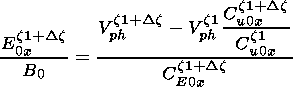Evaluating u_0x^{z 1} from equation (18) for V_ph^{z 1}

(20)

we then substitute it into equation (18) for V_ph^{z 1 - D z}, from which we now can find the other contributor (for this particular case, the meridional neutral wind velocity u_ny^{z 1 - D z} )

(21)

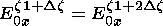
[55]  Then we assume that for the altitude one step down, z 1 - 2 D z, the meridional wind remains the same:

(22)

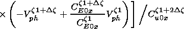
[56]  This allows us to find the polarization electric field at the altitude z 1 - 2 D z from equation (18) for V_ph^{z 1 - D z}

(23)

and so on.

[57]  Note that going up in altitude from the boundary condition with a step D z (altitude resolution of the radar) and applying the same scheme allows reconstruction of the zonal large-scale ( E_0x ) and polarization ( u_0xB₀ ) electric fields. Written in terms of velocity they are:

(24)

(25)

(26)

[58]  It should be mentioned that with each subsequent step down/up in altitude the uncertainty of the method will grow. It is possible to diminish this increasing error in cases when backscatter is observed over a wide altitude range and the data allow us to find two or more boundary conditions, i.e. for the data sets in which there are two or more altitudes where only one contributor defines the phase velocity. Then the contributions may be found using a combination of upward and downward step-by-step evaluation as described above with the obligatory match to the clear boundary condition.

[59]  Obviously the above procedure cannot be used if backscatter comes only from altitudes where two contributors are equally important, since otherwise we would not be able to find the boundary condition.

[60]  In reconstructing the neutral winds and electric fields, we calculate each of the coefficients C_j^{z1 m s D z}, where s = 1, 2, 3, ..., for the time and location of each backscatter event using the altitude dependences of the collisional and gyrofrequencies, which we have found from formulas and the MSIS E 90 and IGRF models.

[61]  Finally, we have had to make some assumptions on the primary waves. Since our method is based on the expression for the line-of-sight Doppler velocity which, unlike the signal power [Hocking, 1985], does not depend on the primary wave spectrum, the polarization electric field is influenced only by the relative density fluctuation in the primary wave but not the primary turbulence scale. On the basis of observations at middle and equatorial latitudes, we suppose that this relative plasma density fluctuation in the primary wave n_pr is 5%. We think that this assumption is reasonable, since numerical studies by McDonald et al. [1975] showed that the generation of secondary small-scale gradient drift irregularities with l <28 m were excited when the amplitude of the larger-scale primary waves exceeded 4% of the background plasma density. Also midlatitude rocket observations [Bowhill, 1966; Itoh et al., 1975; Kelley et al., 1995] showed that n_pr was correspondingly 5-10%, 1-5% and 7%.

Figure 4

[62]  Note, that the reconstruction procedure assumes that n_pr is constant. In fact there is a possibility that n_pr may vary along the radar line of sight (several ionization clouds in the radar field of view). Since C_u0x is assumed constant for the given altitude and time, in the case of variations of n_pr along the radar line of sight relative to the supposed n_pr⁰ = 5%, our method will produce a sinusoidally modulated polarization electric field. In fact, it is possible that precisely this very rare case of three ionization clouds can be seen in the altitude range 100-103 km near 0253 AM LT (section 4, left top and middle panels in Figure 4).

3.2.3. Requirements of the method.

[63]  Summing all the above, we may formulate the necessary conditions for the use of the proposed method as follows: (1) in the backscatter data there should be at least one altitude at which only one contributor defines the phase velocity (the boundary condition); (2) the coefficients C_j change with altitude fast enough to be noticeably different at two neighboring altitudes separated by the altitude resolution of the radar; (3) backscatter should be observed from at least 3 neighboring altitudes; and (4) the altitude resolution of the radar should be good enough to provide reasonable resolution of the winds and electric fields.