3. Mathematical Formulation of the Problem
[10] We chose the spherical coordinate system
Q, j, r, the
Q=0 axis passing through the vertical dipole. The source
excites the falling field independent of
j, so in the
chosen model of a one-dimensional irregular waveguide we have an
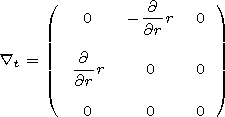
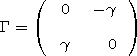
axis-symmetric problem. We write the Maxwell equation in the
matrix form
[Felsen and Marcuvitz, 1973;
Lutchenko and Bulakh, 1986],
taking the following dependence on time
exp(-iwt):
 | (1) |
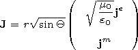
where
E is the electric field intensity vector
(V m-1 ),
H is the magnetic field intensity
(A m-1 ),
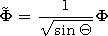
H = (m0/e0)1/2H(sinQ)1/2,
m0 and
e0 are the magnetic and dielectric constants of
the vacuum, respectively,
E = E(sinQ)1/2,
 | (2) |
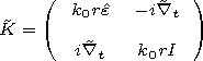
I is a unit matrix,
k0 is the wave number in
the vacuum
k0=w(e0 m0)1/2, e is the dimensionless tensor of the
dielectric permittivity of the magnetoactive medium depending on
r and
Q,
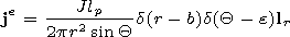
jm is the density of the external magnetic
current,
je is the density of the external electric
current (A m-2 ) and in the case of a vertical point-like
electric dipole located over the Earth surface at
r=b
J is
the current at the antenna input,
lp is the antenna virtual
height, and
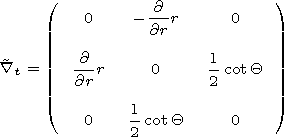
lr is a unit vector. The problem solution
F has to satisfy the impedance boundary
conditions at
r=a, the conditions of a field decrease at
Im k0 > 0 and
r
 , and
its boundedness at
Q=0 and
Q=p. In the accepted model
Im k0 = 0, however for
choosing the solution, the commonly accepted
[Makarov et al., 1993]
principle of the limiting amplitude
in which a presence of losses in the medium leading to
Im k0 > 0 is used. After construction of unambiguous solution,
we come back to the model
Im k0 = 0 and
e = 0.
, and
its boundedness at
Q=0 and
Q=p. In the accepted model
Im k0 = 0, however for
choosing the solution, the commonly accepted
[Makarov et al., 1993]
principle of the limiting amplitude
in which a presence of losses in the medium leading to
Im k0 > 0 is used. After construction of unambiguous solution,
we come back to the model
Im k0 = 0 and
e = 0.
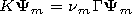
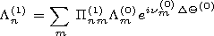
[11] The solution of system (1) is constructed by the cross-section
method
[Katsenelenbaum, 1961],
presenting the solution in
the form of the expansion in terms of orthogonal system of
functions
Ym
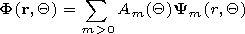 | (3) |
As
Ym, the
eigenfunctions of the lateral operator
K for the regular
waveguides of comparison are chosen. The waveguides of comparison
are spherical waveguides with the polar axis coinciding with the
axis of the initial waveguide and the dielectric permittivity
e(r) which depends only on the coordinate
r and coincides to the dielectric permittivity of the initial
waveguide in the
Q cross section. To construct the
eigenfunctions in the regular waveguides of comparison, we
consider homogeneous Maxwell equations and take approximately that
( dAm/dQ)=inmAm,
where
m is the number of the
mode. Then we neglect
cot Q in the operator
 t assuming that
cot Q
t assuming that
cot Q  nm , ( nm
  k0a).
k0a).
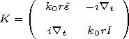
 | (4) |
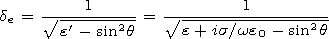
with the boundary conditions
q is the incidence angle of the plain wave on the
Earth surface;
e is the relative dielectric
permittivity of the Earth surface,
s is its conductivity in S m-1,
and by the condition
Ym(r) 0 at
Im k0 > 0 and
r,
G have the form (2).
In real conditions (except the Antarctics, Greenland and the
permafrost regions)
e
 sin2q, so
de with a high accuracy
does not depend on the spectral parameter. Equation (4) is an
equation for the eigenfunctions. In order to obtain the
orthogonality relation for the eigenfunctions a scalar product is
introduced and the conjugated operator
K+ is determined in the following way
sin2q, so
de with a high accuracy
does not depend on the spectral parameter. Equation (4) is an
equation for the eigenfunctions. In order to obtain the
orthogonality relation for the eigenfunctions a scalar product is
introduced and the conjugated operator
K+ is determined in the following way
 | (5) |
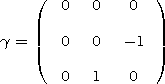
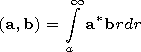
The vector standing at the first place is taken with the complex
conjugation and the parenthesis mean a scalar product
Relation (5) takes place at
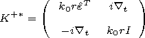 | (5') |
eT is the transposed tensor
e with the boundary conditions
the
sign
 designates a complex conjugation. The eigenfunctions
of the adjoined operator satisfy the equation
designates a complex conjugation. The eigenfunctions
of the adjoined operator satisfy the equation
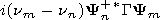
 | (6) |
the eigenvalues of
equation (4) at the same indices coincide with the complex
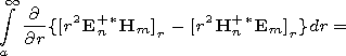
conjugated value of equation (6). We multiply the left-hand side
of (4) to
rY+n, and the right-hand side of
(6) to
rYm and subtract
the latter from the former. Then
or
We integrate both sides of
the latter equality forming a scalar product
where
 | (7) |
Em= ( Em/nm) and
Hm=( Hm/nm) are derivatives with respect to
the spectral parameter and
Nm is the normalizing
multiplier. Expression (3) for the solution we substitute into the
initial equation (1) outside the sources region and multiply its
left-hand side scalarly to
Y+n. Then we obtain
Em/nm) and
Hm=( Hm/nm) are derivatives with respect to
the spectral parameter and
Nm is the normalizing
multiplier. Expression (3) for the solution we substitute into the
initial equation (1) outside the sources region and multiply its
left-hand side scalarly to
Y+n. Then we obtain
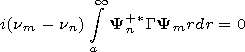
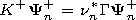
 | (8) |
The solution of the homogeneous equation (8) has an exponential
dependence on the
Q coordinate. At the same time, it is
known that in a regular waveguide, the angular dependence of
normal waves is described by the Legendre function. Only while
using asymptotic presentations of these functions in the wave zone
relative to the source and its antipode, the Legendre function
becomes approximately exponential. Therefore we obtain the limits
of applicability of the solution (3)
cot Q nm or
Q (1/k0a) and
p - Q (1/k0a),
because
nm  k0a.
k0a.
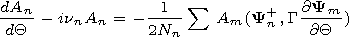
[12] Assuming the eigenfunctions to be normalized, i.e.,
Nn=1, rewrite equation (8) with respect to a new function
Ln(Q) outside the source area for a path
segment, within which the waveguide characteristics are supposed
constant. Let's denote
Q0 the initial coordinate of
such a segment. Assuming the eigenfunctions to be normalized,
i.e.,
Nn=1, we rewrite equation (8) with respect to a new
function
Ln(Q) outside the sources for that part
of the path within which the characteristics of the waveguide are
considered to be constant. Let us designate the initial coordinate
of such part as
Q0.
 | (9) |
 | (9') |
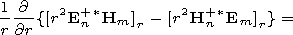
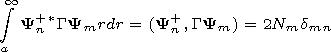
The scalar product
(1/2)(Y+n, GYm/ Q)=Smn describes the differential matrix of
transformation of normal waves
[Lutchenko et al., 1986].
In
the real conditions, the electric properties of the ionosphere
vary smoothly, so the
Smn elements only due to the
ionosphere would be continuous functions of the
Q argument.
However variations in the conductivity of the lower boundary (in
terms of the scales of field changes) in the accepted model occurs
in a jump-like way.
[13] Let a jump-like change of the medium properties occurs in the
cross section with a coordinate
Q0. We designate
F(1) field in the cross section
Q0 - e and
F(2) in the cross section
Q0 + e. The tangential components of the
vectors
GF(1) = GF(2) should be continuous or
 | (10) |
In the
former sum, generally speaking, there should present positive and
negative indices
m ( m < 0 corresponds to reflected waves). We
multiply scalarly (10) to
Yn(2)+. Then
 | (11) |
In the obtained sum
Am(1), amplitudes of reflected waves
m < 0 are unknown, however if we neglect them, the passed waves
are determined in (11) and
An(2)(Q0) = Ln(2).
[14] The scalar product
 | (12) |
may be
interpreted as an element of the matrix
P of transformation of
normal waves and the aggregate
L(2)n may be
considered as the
L(2) vector which is
determined by the product of the
P matrix to the
A(1) vector in the cross section
Q0.
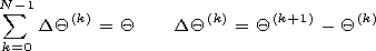
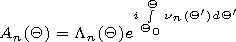
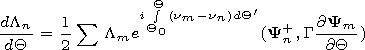
[15] The solution of system of differential equations ( 9' ) presents a
rather tiresome problem, so we will approximately take that the
ionosphere is changing in a jump-like way. A sequence of cross
sections is chosen along the path. In each cross section,
characteristics of normal waves are determined and to the next
cross section the waveguide is considered as homogeneous. At the
joints of the cross sections, the matrix
P is calculated
neglecting the reflected waves. Thus in the
source vicinity, normal waves with the amplitudes
L(0)m are excited. At the next cross section
located at the angular distance of
DQ(0) the
waves will have amplitudes
A(0)m=L(0)m ein(0)mDQ(0). In the next cross
section the amplitudes will be
and so on.
 | (13) |
We
write the solution of system (1) in the form
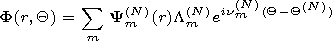 | (14) |
We
determine the coefficients of normal wave excitation by a vertical
dipole assuming that in the vicinity of the dipole
Q (l/ a) the
waveguide is homogeneous and so we use the regular waveguide
model. The methods of calculation of the excitation coefficients
are described below.
(l/ a) the
waveguide is homogeneous and so we use the regular waveguide
model. The methods of calculation of the excitation coefficients
are described below.

Powered by TeXWeb (Win32, v.2.0).