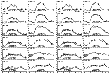
Oblique chirp sounding and modeling of ionospheric HF...

3. Observational Results

Figure 4

[20] Figure 4 shows the results of the processing of oblique sounding ionograms obtained in 2005 at paths of various length and orientation. Each picture corresponds to monthly continuous observations and contains data for not less than 6000 sounding sessions. Using the algorithm developed by Vertogradov [2005], the values of MOF for each session were determined automatically in real time. Thick line in the plots presents the result of the monthly statistical averaging. Together with estimation of the mathematical expectation, the estimate of the standard mean deviation from the mathematical expectation was found. Thin dashed lines in the plots limit the band in the vicinity of the mathematical expectation, the width of the band being equal to the standard deviation doubled. The forecasted value of the maximum usable frequency (MUF) for the corresponding path was calculated for the middle of each month. The MUF was calculated by the x mode. Simultaneously the model IRI-2001 was corrected by the index of solar activity. The effective values of W_eff were used as the index of solar activity [Secan and Wilkinson, 1997]. The values of W_eff for each month are shown in Figure 4. The forecasted values of MUF obtained in the above described way are shown in Figure 4 by crosses.

[21] On the basis of the processing of continuous diurnal dependencies of MUF obtained in 2005, one can draw the following conclusions.

[22] The MOF values for some propagation modes undergo short periodic variations with quasi-periods of ~20 min to 1.5 hours. In quiet ionospheric conditions in the afternoon hours of the day, the fluctuation amplitude can reach 2 MHz. In separate days in dawn-dusk hours at passing of the terminator, the fluctuations at the Cyprus—Rostov-on-Don path can grow up to 5-8 MHz.

[23] At monthly averaging the standard deviations (SD) of MOF from the mathematical expectation at paths of all lengths are higher in the daytime and increase with a path length increase. The typical SDs of MOF in the daytime for various paths have the following values: 1.2 MHz (Cyprus—Rostov-on-Don), 1.7 MHz (Inskip—Rostov-on-Don), 2.0 MHz (Norilsk—Rostov-on-Don), 2.2 MHz (Irkutsk- Rostov-on-Don), and 2.5 MHz (Magadan—Rostov-on-Don). At night SD of MOF decreases (very weak dependence on the path length is still left) down to the following values: 1.0 MHz (Cyprus—Rostov-on-Don), 1.5 MHz (Inskip—Rostov-on-Don), 1.5 MHz (Norilsk—Rostov-on-Don), 1.5 MHz (Irkutsk—Rostov-on-Don), and 1.6`MHz (Magadan—Rostov-on-Don). No seasonal dependence of SD of MOF was found on the basis of the measurements at the Cyprus—Rostov-on-Don and Inskip—Rostov-on-Don paths. Thus the mean diurnal variations of MOF about 1.5-2.5 MHz in the vicinity of the maximum values of MOF (in the daytime) and about 1.0-1.6 MHz in the vicinity of the minimum values of MOF (at night) should be taken as typical values for midlatitude paths of various length in quiet geophysical conditions.

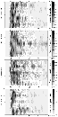
[24] As it has been already mentioned above, MOF of the 1F mode undergo quasiperiodical variations observed almost permanently at various paths. At long multihop paths this effect is partly masked due to high diffusity of the signal caused by the reflection from the Earth and the scattering in the ionosphere. The most distinct variations in MOF were observed at the Cyprus—Rostov-on-Don path 1440 km long. We performed an analysis of these variations aimed at detecting the spectral composition of MOF fluctuations. Two approaches were applied to get rid of the diurnal trend in the time series of MOF. In the first approach, the trend was found by a running averaging at the chosen width of the time window DT. Then the trend was withdrawn from the initial time series of MOF. Such procedure is equivalent to high-frequency filtration. It is not optimal due to high sidelobes of the digital filter. As a consequence the time series of MOF fluctuations save traces with quasi-periods exceeding considerably the width of the time window. In the second approach, the trend was withdrawn on the basis of a digital high-frequency (HF) filtration of the initial series of MOF. The frequency of the filter cutoff was chosen equal to F=1/DT. The tangent Butterworth filter of the tenth-order was used as the digital filter. This procedure provided effective suppression of the components of the diurnal variations in MOF with frequencies below the cutoff frequency F of the digital filter.

Figure 5

[25] The spectral analysis was performed using the fast Fourier transform (FFT) algorithm. The examples of the spectral density for the Cyprus—Rostov-on-Don path for a series of consequent days of various months are presented in the form of sonogram in Figure 5. Analyzing the graphs of the spectral density of the power of MOF fluctuations, one can conclude the following:

[26] 1. For different seasons the spectra of the MOF fluctuations have a well-pronounced linear structure, this fact manifesting that the MOF fluctuations are due to propagation in the ionospheric plasma of a train of quasi-harmonic waves.

[27] 2. The power of spectral components of MOF fluctuations is concentrated in the 20-90 min range.

[28] 3. The spectral composition of the MOF fluctuations varies from one day to another, though some quasi-harmonic components can exists in MOF fluctuation spectra during a few days.

Figure 6

[29] In order to reveal the main quasi-periods of MOF fluctuations, the results of the spectral processing were subjected to a statistical analysis. To do that, in each spectrum (for a day) 5 the most intense harmonics were chosen and used to determine the corresponding quasi-periods. Then, using the monthly data obtained, the histograms of distribution of quasi-periods at the Cyprus—Rostov-on-Don and Inskip—Rostov-on-Don paths were drawn. The histograms are shown in Figure 6.

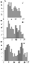
[30] The results obtained make it possible to draw the following conclusions.

[31] 1. The most probable quasi-periods for both paths are concentrated within the 20-90 min interval.

[32] 2. The positions of maximums and their number change from one month to another.

[33] 3. The most high-frequency component in the fluctuation spectrum has a quasi-period in the vicinity of 15 min and is present at both paths in all seasons, though the amplitude of this quasi-harmonics varies from one month to another.

[34] Fluctuations of MOF are accompanied by appearance the z-type features in frequency-time display ionograms (see Figures 2 and 3) what appear in the vicinity of the lowest observed frequency (LOF) for the high-angle rays and drift with time to the region of lower delays (into the vicinity of MOF). These features were observed in various time of the day at all paths where the observations were conducted. However, most often and with maximum amplitudes, the z-type features were registered at the one-hop paths Cyprus—Rostov-on-Don and Inskip—Rostov-on-Don at dawn-dusk hours of the day at the passage of the terminator. Typical amplitudes of z-type features at frequency-time display achieve values ~0.1-0.5 MHz. On the basis of modeling, we will show below that the z-type features are due to the motion of traveling ionospheric disturbances (TID). At lower amplitudes of TID, breaks and steps of various amplitudes are observed in frequency-time display. We analyzed the appearance of TID detected by means of the high-angle ray and found their period for the Cyprus—Rostov-on-Don path where this effect was manifested most visually. The period of TID responsible for formation of z-type feature was detected from the frequency-time display ionogram analyzing the time interval between appearance at low frequencies of the high-angle ray of z-type feature, their drift along the track from low to high frequencies, and appearance of the wave train at low frequencies immediately after disappearance of the previous train of wave disturbances at high frequencies in the vicinity of MOF. If on the track of the high-angle ray one more z-type perturbation appears, this causes the uncertainty in the TID period determination. We exclude such cases from our consideration. The detected in such a way typical values of the TID periods were ~15-30 min.

Figure 7

[35] Figure 7 shows a histogram of the distribution of probability of TID appearance with time of the day for various months of 2005 according to the data of the oblique LFM sounding of the ionosphere at the Cyprus—Rostov-on-Don path. Vertical dashed lines show the sunrise and sunset for the middle point of the path for the 15th day of each month. Different time interval of signal registration in different months is due to the fact that the LFM transmitter at Cyprus starts from the frequency of 8 MHz which exceeds MOF at the Cyprus—Rostov-on-Don path at near-midnight hours for February (March). One can see in Figure 7 that the appearance of TID with periods 15-30 min correlates well with the dawn and dusk for the middle point of the path. At dawn-dusk hours the probability of TID appearance reaches 80-100%. These data confirm the important role of terminator as a source of TID generation.

[36] The traces of one-hop propagation modes (the Cyprus—Rostov-on-Don and Inskip—Rostov-on-Don paths), as a rule, have no indications to diffuse reflections and look like thin lines, their thickness being comparable with the Rayleigh limit of the spectral analysis. The traces of multiple modes have some indications to diffuse reflections. The latter fact is, evidently, due to the scattering at the reflection from uneven surface of the Earth. This statement is confirmed by the observations at the Cyprus—Rostov-on-Don path. The region of the arrival of the first hope for the two-hop mode falls there at the sea-land boundary (the Black Sea coast of Turkey). As a rule, the 2F mode at this path demonstrates well-pronounced traces of diffusivity (see Figures 2 and 3b), this fact being, evidently, due to scattered reflection from the mountain Earth surface. At the same time, sometimes a clear trace of the 2F mode appears for a short period (see, for example, Figures 3c and 3d). This trace looks like the one for the 1F mode. The latter fact is, apparently, a result of the reflection from the sea surface. This event was observed at neither of the paths Inskip—Rostov-on-Don, Irkutsk—Rostov-on-Don, Norilsk—Rostov-on-Don, and Magadan—Rostov-on-Don. The multiple modes at these paths always have signs of diffuse reflections, the diffusivity degree increasing with an increase of the mode order.

[37] The frequency-amplitude display of some propagation modes show deep fluctuations (up to 20-30 dB, see Figures 2 and 3). The quasi-period and fluctuations depth vary with the frequency. Generation of the fluctuations can be explained by interference of nonseparated rays within one propagation mode. In this case the depth of the fluctuations and quasi-period are determined by the relation between the ray amplitudes and the difference in the group delays, respectively. It is known that, with the accuracy to linear terms, the signal phase may be presented in the form

(1)

where f₀ is the initial phase, df is the Doppler shift of the frequency, and t is the group delay. One can see that the quasi-period of amplitude fluctuations is determined by the difference in the group delays of the nonseparated partial rays. Evidently, the zero beats will be observed, that is the fluctuation period will increase strongly, where the group delays of the rays coincide. This is observed in the region of the crossing of two magneto-ionic components at frequency-time display (see Figures 2 and 3).

[38] In the region where the magneto-ionic components are separated and only the trace of the extraordinary wave is left, the interference fluctuations at frequency-amplitude display almost disappear (one-ray propagation).

[39] In the vicinity of the dead zone at frequency-amplitude display of partial rays an effect of focusing is observed. The value of the focusing can reach 10 dB. Similar effect takes place in the vicinity of the "noses'' of z-type features at frequency-time display.

[40] This regular behavior of frequency-amplitude display of particular propagation modes and rays can serve as a proof of the dominating propagation mechanism in the form of discrete rays (mirror components). A casual input into the initial phase in (1) due to small-scale structure of the ionosphere appears to be small and insignificant. In the opposite case, the random fluctuations at the amplitude display would have been observed. Just so looks the amplitude display of multiple propagation modes.