Extreme solar events and magnetic storms in October 2003 and...

2. Estimate of the Variations in the Electron Concentration in the Ionospheric shape D region Using VLF Signals Observation Data

[4] To analyze variations of the structure and dynamics of the lower ionosphere during solar events and magnetic storms on 28-30 October 2003, signals of the phase radio direction finding system (PDFS) "Alpha" operating at frequencies of the VLF range (11.9, 12.65, and 14.9 kHz) were used. The master station is located in Novosibirsk, whereas the slave stations are located in Khabarovsk and Krasnodar. The reception point is located at the Radio Physics Department of the St. Petersburg State University in Petrodvoretz. The map of the location of the stations and the reception point is shown in Figure 1. The reception of the signals, registration of the amplitudes and phases, and also storage of the information were performed using the original digital received developed in Radio Physics Department of the St. Petersburg University [Belenky et al., 2002].

[5] The master station transmits (besides the working signals) every 3.6 s the data on the absolute phase delays of the signals at a frequency of 11.9 kHz occurring at the Novosibirsk-Krasnodar (the Western Base, WB) and Novosibirsk-Khabarovsk (the Eastern Base, EB) paths in the process of propagation. This information is also used for the analysis of the ionosphere dynamics at the propagation paths.

[6] Figure 1 shows the paths Novosibirsk-St. Petersburg (path 1) and Krasnodar-St. Petersburg (path 2). All the above indicated paths are located at middle latitudes and that makes it possible to observe the southward shift of the auroral processes and processes of energetic electrons injection into the D region during the magnetic storms on 29-30 October 2003. The Western Base, Eastern Base, path 1, and path 2 are located between 41^o and 44^o, 38^o and 46^o, 44^o and 57^o, and 41^o and 56^o geomagnetic latitude, respectively. Thus WB and EB make it possible to observe the injection of charged particles into the ionospheric D region at geomagnetic latitudes 41-46^o in two longitudinally separated regions.

[7] The timescale of the reception point is not synchronized to the scale of the master station and it follows that the measurements of absolute delays of the signals phases on path 1 and path 2 are impossible, only their variations during a day can be determined. Moreover, a discrepancy between the ratings of the frequencies of reference generators at the transmitting station and reception point is possible. This discrepancy may be compensated by statistical processing of values of the received phases.

Figure 2

[8] The variations of the electron concentration in the ionospheric D region were estimated comparing the variations in phases and amplitudes obtained in calculations with modified model vertical profile of the electron concentration and the observed variations in phases and amplitudes of the received signals on path 1 and path 2 and the data on the phase delays at the bases. In these calculations the standard model of the lower ionosphere created by Azarnin et al. [1987] was taken as a model for undisturbed conditions. The model takes into account dependence on geomagnetic latitude, local time, solar zenith angle, season, and solar activity phase. The N₀(z) model above 75 km coincides to the known International Reference Ionosphere Model IRI [Bilitza, 1990]. The lower part of the profile is fitted in such a way that the calculation results of the fields and reflection coefficients from the ionosphere correspond to the published experimental data in the VLF range in undisturbed conditions. Similar method of profile creation was described earlier [Rishbeth and Garriott, 1969]. Figure 2 shows typical vertical profiles of the model electron concentration N₀(z) in undisturbed conditions in Novosibirsk on 29 October 2003 at 0600 UT (day) and 1800 UT (night), and also during a dawn at 0235 UT and dusk at 1010 UT. Modification of the model for disturbed conditions included correction of its parameters till the best agreement between the calculated and observed variations of the phases and amplitudes of the fields of VLF radio signals propagating in the Earth-ionosphere waveguide channel. The disturbed profile was described by the function

This function makes it possible to describe variations in both D and C layers of the ionosphere by selection of the values of the p, q, z₀, and Dz parameters. The p parameter influences the height of the region significant at the propagation and determines the phase of the VLF signal. The parameter q less influences the phase, but changes considerably the amplitude at 50

z₀

55 km and 5

10 km.

[9] For illustration of the influence of parameters p, q, z₀, and Dz, Table 1 shows the results of the calculations of the amplitude (mV m ^-1 ) and phase (in degrees) of the signal at path 1. The current in the transmitted antenna was taken independent on the frequency. The first line p=1 and q=0 corresponds to the corresponding undisturbed state of the ionosphere at 1100 UT in October 2003.

[10] A similar model of disturbed ionosphere containing an exponent was used earlier for studying of the regions in the ionosphere determining the reflection coefficients [Wait and Walters, 1963] and regions important for propagation of VLF [Orlov and Uvarov, 1975].

[11] The calculations were performed using the programs developed by L. N. Loutchenko and M. A. Bisyarin (submitted to Int. J. Geomagn. Aeron., 2006). Using the given coordinates of the receiver and transmitter, the program calculates the geodesic, find coordinates of intermediate points along the path. Using these points and the taken map of conductivity of the Earth soil, the conductivity in these points is found. Using the date and time N₀(z) in each point is detected. The paths WB, EB, and path 1 have a length more than 3000 km, so in the daytime the signals are determined by one mode. Several modes should be taken into account at night. The length of the path 2 is about 1700 km, so higher modes influence variations in the phase and amplitude even in the daytime. The interference of modes propagating with different velocities and depending on the frequency explains different behavior of the amplitudes at different frequencies in disturbed conditions and under varying illumination at path 2. The information obtained from the above described experiment is not sufficient for solution of the inverse problem of creation of a spatial-time model of the disturbed ionosphere and unambiguous determination of its parameters. The aim of this paper is only to estimate an order of magnitude of the electron concentration variations caused by the solar flare and to follow the development of the ionosphere-magnetosphere disturbances.

[12] The prominent solar flare X17.2/4B began on 28 October 2003 at 0951 UT was registered by GOES 10 satellite and was accompanied by the X-ray emission in the range 1-10 Å and by powerful radio bursts of all types, and also by acceleration of charged particles up to 7 GeV. The flare maximum was registered at 1110 UT.

Figure 3

[13] Figure 3 shows the data on the reception of VLF signals on 28 October 2003. Figure 3a shows the diurnal variations of the phase at a frequency of 11.9 kHz at WB and EB (Figure 3b). Below are shown the values of phases and amplitudes at the working frequencies at path 1 (Figures 3c and 3d), and path 2 (Figures 3e and 3f). The variations of radio signal parameters were compared with the variations of the AE index presented in Figure 3g for 28 October. It follows from Figure 3 that at the sunlit path WB, path 1, and path 2 there occurred a sharp decrease of the phase synchronously with the maximum of the flare, whereas at EB only some slowing down of the development of the transition to the nighttime values of the phase was observed. Similar increase of the electron concentration in the D region in the nighttime hemisphere of the Earth a few minutes after a prominent flare was noted earlier by Rishbeth and Garriott [1969].

Figure 4

[14] For interpretations of the above mentioned features in the VLF signals, Figure 4 shows solar zenith angles c calculated for the intermediate observation points approximately with a step of approximate 250 km along the WB, EB, path 1, and path 2 for 1000 UT and 1110 UT. It is worth noting that the ionosphere region at heights of 50-90 km is important for propagation of VLF signals. The solar zenith angle c =99.6^o and c =97.2^o correspond to the position of the low boundary of the sunlit region at 90 and 50 km, respectively. Thus, at c<97.2^o the entire region important for the propagation is sunlit, whereas at c >99.6^o the entire region is in the dark. Thus, at 1000 UT a half of EB is in the shadow. At 1110 UT already 80% of EB are in the shadow and so the X-ray flux disturbs only a small portion of the path. The other path is completely sunlit. The phase at WB decreased by 10 centicycles (cc) at 1000 UT. At 1110 UT it decreased by 25 cc more (see Figure 3a). Such variation in the phase may be caused by an increase of the electron concentration. The calculations show that to reduce the phase by 10 cc one has to increase the electron concentration by a factor of 2.5 ( p=2.5 ). To have a reduction by 30 cc, one needs an increase of N₀(z) by a factor of 20 ( p=20 ). Similar increase in the electron concentration in the ionospheric D region was measured during prominent flare by the partial reflection method by Belrose and Cetiner [1962]. The disturbed profile N(z) at p=20 is shown in Figure 2.

[15] At path 1 at 1110 UT the phase decreased approximately by 25 cc at all three frequencies. The amplitude increased by 0.3 dB and decreased by 0.5 dB at frequencies of 14.9 kHz and 11.9 kHz, respectively. One can obtain such variations in the fields using the model of N(z) with p=5 and q=10 cm^-3, Dz=10 km, z₀=55 km.

[16] At path 2 the phase decreased approximately by 20 cc at all frequencies. The amplitude increased by 0.6 dB at a frequency of 14.9 kHz and was unchanged at two other frequencies. Calculations provide such variations of the field characteristics at p=20 and q=200 cm^-3. Thus, to describe the amplitude variations one has to choose models with increased electron concentration in the D region below 60 km (the region often called as the C layer).

Figure 5

[17] Figure 5 shows the graphs for 29 October 2003 similar to Figure 3. It follows from Figure 5 that at 0440 UT a sharp decrease of the phase by approximately 20 cc occurred synchronously at WB and EB with a maximum at 0500 UT. It should be noted that at 0440 UT the GOES 10 satellite registered X-ray emission from the solar flare of the M3.7 class; however, no phase disturbances are seen at this time neither at path 1 nor at path 2.

Figure 6

[18] The intensity of this flare is by about a factor of 50 lower than the intensity of the flare on 28 October; however, the response of the VLF signals phase at WB is weaker only by a factor of 1.7. We compare the observed effect with the phase response dependence on the intensity of the X-ray flux for other solar flares. 88 sudden phase anomalies were registered at WB and EB with the help of the above described receiver in 2001 and 2002 from April to August. The intensity of the X-ray flux was taken according to the data of the GOES satellite (http://www.sec.noaa.gov/ftpdir/indices/SPE.txt). The deviations of the phase value at WB and EB are presented in Figures 6a and 6b, respectively, as a function of the decimal logarithm of the flare intensity normalized to 1 W m ^-2. Large squares in Figures 6a and 6b correspond to the events on 28 and 29 October. One can see that within the scatter of the phases which may be explained by differences in the X-ray spectra for different events, the observed disturbances in phase at WB and EB on 28 and 29 October agree well with other observations.

Figure 7

[19] Now we discuss the cause of the absence of the response of VLF signals at path 1 and path 2. Figure 7 shows the solar zenith angles at 0500 UT on 29 October along WB, EB, path 1, and path 2. One can see that along the entire path 2 the solar zenith angles exceed 81^o and more than a half of path 1 also has c >80^o. To make the comparison of illumination of path 1 at 1110 UT on 28 October and at 0500 UT on 29 October more convenient, both graphs are shown in Figure 7. One can see that the range of c variations is the same in the both cases. The only difference is that the conditions on 28 October and 29 October correspond to the dusk and dawn, respectively. Azarnin et al. [1987] noted that the standard model of the electron concentration N₀(z) at c >80^o is considerably different at the dawn and dusk (see Figure 2), so the same additional ionization by X rays provides different response of VLF signals. For example, the calculations using the N(z) model with p=1 and q=30 cm^-3 give a decrease of the phase at path 1 by 2 cc and 10 cc at 0500 UT and 1110 UT, respectively. These values agree with the experiment if one takes into account Figure 5 and the increased intensity of the X-ray radiation on 28 October.

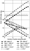
[20] Interplanetary shock wave reached the Earth on 29 October at 0612 UT [Panasyuk et al., 2004]. However, sharp changes in the signals at path 1 on 29 October were observed only at 0640 UT (see Figures 5c and 5d). The phase decreased approximately by 30 cc at all three frequencies and the amplitude at 0700 UT decreased by 2 and 0.5 dB at frequencies of 11.9 and 14.9 kHz, respectively. One can obtain such variations in the fields in simulations using the model with p=5, q=150 cm^-3, Dz=10 km, and z₀=55 km.

[21] The sharp changes in the signals continued later approximately at 0915 UT, 1020 UT, and 1120 UT at all three frequencies with the maxima at 0700 UT, 1030 UT, and 1145 UT, the effect decreasing with a frequency increase. One can see in Figure 5g that the above indicated time intervals coincide with sharp increases in the values of the AE index exceeding 1500 nT. Therefore the sharp variations of the phases are related in this case to variations in the electron concentration in the D region caused by development of auroral processes.

[22] At path 2 a sharp decrease in phase by about 10 cc was observed at 0700 UT (Figures 5e and 5f). This decrease corresponds to the model with p=3, q=50 cm^-3, Dz=10 km, and z₀=55 km. Then the decreases were repeated with a quasi-period of 30-40 min and amplitudes of about 5 cc. That may be related to strong chaotic variations of the electron concentration around the increased (on the average) level of the latter.

[23] The propagation conditions at WB were close to undisturbed conditions from 0600 UT to 2000 UT (Figure 5a) and then sharp changes in the phase up to 15 cc were observed. The changes were related to the increase of the electron concentration at night at about 2000 UT and 2300 UT. At EB (Figure 5b) the nighttime conditions from 1400 UT to 1700 UT were disturbed relatively weakly (the phase decreased by 10 cc), whereas at 1700 UT a sharp decrease of the phase by 20 cc occurred and it almost reached the daytime undisturbed values (see Figure 3b). The phase was restored to its nighttime value to 1800 UT. Then at about 1830 UT a new decrease to the daytime values began and at 2000 UT the phase reached its maximum value by 5 cc below the nighttime level. A transition to the daytime conditions began already at 2000 UT which is by 2 hours earlier than in usual undisturbed time. Very strong phase and amplitude fluctuations are observed at night at path 1 and path 2 (Figures 5c, 5d, 5e, and 5f). The transition to the daytime conditions began at path 1 by 1 hour earlier than usually.

Figure 8

[24] To analyze further development of the ionosphere-magnetosphere disturbances, we consider Figure 8 where the graphs similar to the above described are presented for 30 October. Figure 8a shows the phase corresponding to the delay of the VLF signals at WB. The character of the phase behavior from 0000 UT to 1200 UT is similar to undisturbed conditions and differs only by an increased level of fluctuations. About 2000 UT quick changes in the phase with the amplitude of about 10 cc appeared. Then at 2100 UT a sharp decrease of the phase by 15 cc which lasted during an hour was observed. Then a slow restoration of the phase began on the background of strong fluctuations. At 2300 UT the phase almost reaching the nighttime values decreased sharply again by 10 cc. To describe the phase depletion at night by 15 cc, one can choose several different models, for example, Dz=10 km and z₀=55 km, (1) p=20, q=2 cm^-3 and (2) p=10, q=10 cm^-3.

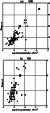
[25] On 30 October in the intermediate conditions of illumination after 1300 UT the amplitude at path 1 oscillated within 2 dB with a characteristic time of about 2 hours at almost undisturbed behavior of the phase. One can describe such a situation by a model with appearing and disappearing C layer at q=0.1 cm^-3.

[26] In the daytime on 30 October the phase at EB (see Figure 8b) was below the undisturbed level by 10 cc (increased electron concentration) and as usual a transition to the daytime conditions began. About 0700 UT the electron concentration stopped to decrease as in undisturbed conditions and during 1.5 hours stayed without changes and then began slowly to transit to the nighttime state. The phase reached the nighttime level to 1500 UT and at 1700 UT decreased by 10 cc. At 1800 UT the phase returned to the nighttime level and then with strong fluctuations began to decrease. To 2000 UT it reached the daytime undisturbed level (see Figure 3b) to 2030 UT increased by 10 cc, then decreased again down to the daytime level to 2100 UT, and did not rise any more. The transition to the daytime conditions usually begins at this path at 2200 UT.

[27] In the daytime conditions on 30 October the amplitude at path 1 was below the daytime undisturbed conditions (Figures 8c and 8d). At 1800 UT (already at nighttime conditions) a sharp decrease of the phase by 15 cc and a decrease of the amplitude occur. One can describe this situation by the N(z) model with p=5, q=1 cm^-3, Dz=10 km, and z₀=55 km. At about 2000 UT the phase fell down below the daytime values then increased by 15 cc and to 2100 UT decreased again below the daytime values and to 2200 UT returned to the daytime values. The transition from the nighttime to the daytime values usually begins at 2200 UT.

[28] The propagation conditions at path 2 were disturbed since 1600 UT (Figures 8e and 8f) and because of the multimode structure of the field that strongly influenced its amplitude. Since 1800 UT the phase fluctuations also were intensified.

[29] The AE index (Figure 8g) exceeds the 2500 nT from 1730 UT to 1800 UT, then sharply decreases and increases again up to 2000 nT at 1900 UT, decreases again, and at 2000 UT increases up to 2500 nT. The precipitations corresponding to such AE index make the nighttime ionosphere at EB and path 1 almost similar to the daytime one (see Figure 2).