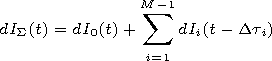
Localization of the source of ionospheric disturbance...

3. Method of Determination of the "Switch-on Time" and Localization of the Secondary Source of the Ionospheric Disturbance Generated During the Earthquake

[31] Now we consider the complex method proposed by the authors of determination of parameters of the disturbance wave front in the near and remote zones of the source using GPS gratings on the example of the 25 September 2003 earthquake.

Figure 5

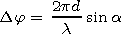
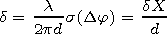
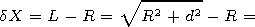
[32] The geometry of determination of wave front parameters using GPS gratings in the remote zone of the source is shown in Figure 5. To simplify the calculations, the latitude and longitude of the subionospheric points is recalculated into horizontal Cartesian coordinates ( x_i, y_i) in the topocentric coordinate system. The center of the system (x₀, y₀) coincides to the coordinates of the point source of the pulse disturbance. This approximation is true for the distances of the subionospheric points from the epicenter considerably less than the Earth radius, this condition being fulfilled in our case.

[33] The X and Y axes are directed eastward and northward, respectively. The concentric circles show the position of the wave front at various moments of time. The diamonds and symbols A₁, B₁, and C₁ and A₂, B₂, and C₂ denote the GPS stations forming gratings R1 and R2, respectively. R₀ and L are radius vectors of points A₁ and C₁, respectively. The line between points A₁ and C₁ with a length of d is a base of an elementary interferometer (phase radar) used for determination of the direction (azimuth) of the wave vector K of the disturbance (the normal to the wave front in the vicinity of points A₁ and C₁ ). The azimuths a₁ and a₂ are marked by dotted arcs.

[34] In the plain front approximation the phase difference Dj of the wave disturbance in points A₁ and C₁ is proportional to sin a:

(1)

where l is the wavelength of the disturbance. In the case when vector K is close to the normal to the position of the base d we write

(2)

In this approximation the error in azimuth calculation d is determined by the increment of the phase difference s (Dj) proportional to the linear deviation dX of the spherical front from the plane front (Figure 5)

(3)

The required accuracy d of the azimuth determination depends on the given accuracy of calculation of the coordinates of the source DR:

(4)

Formulae (4) provides an evaluation of the maximum permitted deviation DX

(5)

On the other hand, if the base d is small as compared to the distance R to the source ( d²

R₀² ) (Figure 5), then

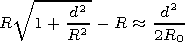(6)

[35] In this case the distance to the remote zone should be larger than

(7)

For the relative accuracy d=0.05 and base d=100 km the radius of the remote zone should be R₀=1000 km. The accuracy of source coordinate determination is in this case ~50 km. The value R₀=1000 km is close to the dimensions of the aperture of the complete GPS grating of the order of 700 km, i.e., to the maximum dimensions of the spatial distribution of subionospheric points for all GPS stations and all satellites presented in Figure 1. Thus it follows that particular GPS gratings with the base shorter than 100 km (for example, MIZU, USUD, and TSKB; PRN 13 and USUD, KGNI, and KSMV; PRN 24, see Figure 1) may be used for determination of the direction to the source in the approximation of a plain wave. The presented below evaluations of the disturbance phase velocity in the approximation of a plane front for various combinations of GPS gratings consisting of three stations were obtained using the SADM-GPS method [Afraimovich et al., 1998, 2001b, 2004].

[36] The entire set of the GPS stations presented in Figure 1 is located within the near zone of the source, because for the total aperture of about 700 km at the same requirements to the accuracy of source coordinate determination d=0.05 the distance to the remote zone is 7000 km. Therefore for joint processing of the data of the total GPS grating one should use the approximation of the spherical front [Afraimovich et al., 2001a].

[37] We use a simplified model in which the epicenter emitter of SAW during the earthquake is substituted by a point-like source of SAW located at a height of h_s in the ionosphere. At h_s=0 km it coincides to the epicenter of the earthquake. The SAW front presents a sphere expanding from the source in the ionosphere with a constant radial velocity V_r. Since only variations of TEC along the "receiver-satellite" ray can be registered at the spatially dispersed GPS detectors, the analysis of the data of GPS gratings makes it possible to evaluate parameters of the wave front only in the horizontal plane. On the other hand, the wavelength of the disturbance is comparable or larger than the scale height of the electron concentration in the F region and the altitude range where AGW still are able to propagate. Therefore in the first approximation the wave front of the secondary disturbance source at the ionospheric level is quite able to be considered as a spherical one.

[38] Moreover, we do not take into account the transformation of the TEC response amplitude to passage of SAW which is determined by the spatial attenuation of the SAW amplitude, aspect relation between the disturbance wave vector, direction to the satellite [Afraimovich et al., 1998, 2004], and orientation of the magnetic field vector [Afraimovich et al., 2001b].

[39] In these conditions the algorithm of spatial-time processing is reduced to summation of the preliminarily phased series dI_i(t) to the reference series dI₀(t). As a result we obtain the total signal of the spatial collection of the TEC series with the remote trend:

(8)

where Dt_i is the time shift of the i th series dI_i(t) relative to the reference series dI₀(t); i=1, 2, 3,...,M, where M is the number of summated series. The time shift is determined experimentally as a difference of time moments of registration of extremes of SAW responses in the i th and background series of TEC with the remote trend:

(9)

As a reference point we take the position of the ionospheric response to SAW with the minimum value of time t_min. For the event on 25 September 2003 the reference point is the subionospheric point MIZU; PRN 13 with the time t_min,0=20.058 UT. Then the time series of TEC with the remote trend dI₀(t) for the GPS station MIZU; PRN 13 we will also consider as a reference series.

[40] Because of the fact that the TEC oscillation caused by the SAW propagation well mutually correlate in each summated series and the background noise oscillation are not correlated (see Figure 3), the signal-to-noise ratio in the total signal of the spatial collection increases not less than by a factor of M^1/2.

[41] Spatial-time processing of TEC series with remote trend is performed in the scope of the model of the spherical front of the ionospheric disturbance wave propagating from a point source in all directions with a constant radial velocity. According to the accepted model, the time shift of the summated series will be determined by the difference of radial distances of the ionospheric disturbance registration points (subionospheric points) from the acoustic impact source (the earthquake epicenter) as well as by the radial velocity of SAW propagation (Figure 5):

(10)

where Dr_i = r_i - r₀ is the difference between the radial distances of the i th and reference subionospheric points from the ID source and V_r is the radial phase velocity of ID.

[42] Consequently, the expression for the radial distance of the i th subionospheric point of the ID source is written as

(11)

where x_i, y_i are the coordinates of the i th subionospheric point in the topocentric coordinate system, h_d is a height above the ionization maximum of the ionospheric F2 layer (i.e., the height where registration of ID occurs), x_s, y_s are the coordinates of the ID source, and h_s is the assumed height of the ID source.

[43] Bearing in mind that the projection of the reference subionospheric point onto the Earth surface (i.e., x₀=0, y₀=0 is the beginning of the chosen topocentric coordinate system, the expression for the radial distance of the reference subionospheric point from the ID source takes the form

(12)

Taking into account (11) and (12) the expression (10) is written in the form

(13)

where i=1,2,3,..., M-1.

[44] Then for the whole set of ID registration points we obtain the system of ( M-1 ) equations:

(14)

[45] An approximate solution of the obtained system relative to x_s, y_s, V_r is found numerically by the random search method under the condition of minimum of the mean square discrepancies s_t of the left-hand and right-hand sides of the equations. The range of looking for the value of each searched parameter and the step of its change are prescribed. For the sake of convenience in the work, the range and step for looking of the ID source location are prescribed in geographical coordinates L_s, and F_s, which are transformed into topocentric coordinates in the process of calculation.

[46] In the search process an exhaust of all possible values of L_s, F_s, and V_r in the given range and with the given step is performed and for each combination of these parameters a value of the mean square of discrepancies s_t is determined. The values of L_s, F_s, and V_r, providing the minimum value of s_t, are taken as a solution of the equation system and therefore the ID parameters looked for.

[47] The calculation of the "switch-on time" of the ID source is performed in the scope of the accepted model of the spherical front on the basis of the calculated source coordinates L_s, and F_s and phase radial velocity V_r taking into account the known time of the registration of the SAW response in the reference point t min,0. In this case the expression for determination of the "switch-on time" of the ID source is written in the following form:

(15)

where r₀ is the radial distance of the reference subionospheric point from the calculated position of the ID source.

[48] The form of the signal of the spatial collection d I_S (t) is an indirect criterion of correct solution of the equation system (12). Such signal for the 25 September 2003 event is shown in Figure 3, panel l. One can see that the amplitude of the summated signal exceeds the amplitude of the reference signal d I_S (t) for the path MIZU; PRN 13 (Figure 3, panel i) almost by an order of magnitude, which corresponds to the total number of paths. Moreover, the TEC variations outside the response are considerably lower then for individual paths, the fact manifesting an increase of the signal-to-noise ratio. The signal of the spatial collection d I_S (t) for the 4 July 2000 event is shown in Figure 3, panel f.

[49] It should be noted that the accuracy in determination of the phase velocity V in the approximation of the plain front is considerably higher than under using the algorithm for the spherical front. In the former case for each GPS station the detection of the disturbance is performed for the same satellite with the same aspect conditions and the velocity of the shift of the reference system, so one has only to take into account this shift in the scope of the SADM-GPS method [Afraimovich et al., 1998, 2004]. In the latter case solution of the equation system (12) is performed relative to the rays to different satellites with different aspect conditions and shift velocities of different reference systems not taken into account in the described method in the first approximation. Though the reference system shift (up to 50 m s^-1 at a height of 400 km at the elongation angles above 30^o) occurs with velocities much slower than the phase velocity V of the wave (1000 m s^-1 ) this error may be only by several times less than the value of V itself. In future a modernization of the method in the approximation of the spherical front is needed taking into account corresponding aspect conditions and shifts of the reference systems for each ray to the satellite.