Application of GEOTIME Computer Environment to Space-Time Modelling of Earthquake Preparation Processes
A. V. Ponomarev, G. A. Sobolev
Institute of Seismology, UIPE, Russian Academy of Sciences, Moscow, Russia
V. G. Gitis
Institute for Information Transmission Problems, Russian Academy of Sciences, Moscow, Russia
Zhang Zchaocheng, Wang Guixuan, and Qin Xinxi
Center for Analysis and Prediction, State Seismological Bureau, Beijing, China
Electronic version of the paper submitted for publishing in Journal of Earthquake Prediction Research
© Copyright 1997 by A. Ponomarev, G. Sobolev, V. Gitis, Zhang Zchaocheng, Wang Guixuan, and Qin Xinxi
© Copyright 1997 by Geophysical Center RAS (electronic version only)
Figures 7, Tables 2
An approach to the space-time analysis of multidisciplinary geophysical observations is
described in relation to the geodynamic process of intraplate earthquake preparation.
The GEOTIME computer Environment is applied to test the hypotheses about earthquake precursors.
The data are processed by three stages: (i) cleaning the time series of geophysical
measurements of seasonal rhythms, non-linear trend, noises and signal standardisation;
(ii) calculation of space-time dynamic fields using the time series from all analyzed
stations; (iii) detection of nonstationarities, estimation of dynamic fields on significance
level, and geophysical interpretation.
Retrospective predictions of Tangshan (July 28, 1976, M = 7.8) and Datong
(October 19, 1989, M = 6.1) earthquakes are considered as an example.
Daily time series obtained from 10 stations since 1972 for Tangshan and from 10
stations since 1981 for Datong were processed to model the process of earthquake
preparation and to detect the earthquake precursors. The suggested space-time approach
is shown to be effective for research on earthquake prediction.
Go to Contents
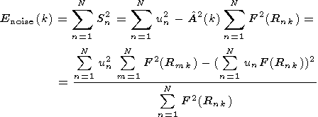
The problem of reliable prediction of earthquakes still remains unsolved in spite of
the tremendous efforts of scientists in many countries. The difficulty is largely due
to the complicated task of identifying earthquake precursors from geophysical monitoring
data.
The obstacles to the solution of the latter problem have several main causes:
- the research cannot be reproduced experimentally in all required conditions, because
the observation of precursors cannot be repeated with recurring parameters of earthquakes
(closely approximating values of hypocenters, magnitude and mechanism of the source);
- the insufficient density and regularity of the geophysical monitoring network to provide
registration of precursors;
- the variations in the tensosensitivity of observation stations in time and space
influenced by the effect on tensosensitivity of geological conditions (faults,
sedimentary cover, hydrological peculiarities), of meteorological factors, and of
stresses in the region of the station;
- the presence in the measured data of the non-linear trend and of the seasonal
rhythms of various periods from cosmic, meteorological and anthropogenic sources;
- the complexity of the model of earthquake preparation, which implies two principally
different types of precursors: 1) those originated in the earthquake focus and 2) those
caused by tectonic environment reflecting the changes in the stress field over a large area;
- the lack of the theoretical image of a precursor appearing in the earthquake focus;
- the activity of trigger effects of different physical nature.
Nonetheless, we may presume on the basis of a vast experience accumulated in many
countries, that precursors were actually observed in a number of cases. On the observation
station, their form can be approximated by several types of signals; i.e., the appearance
of distortion of the trend, the baylike anomaly, the unipolar or double-polar impulse.
It is also assumed that the precursors can occur and disappear repeatedly in the course
of preparation of an earthquake.
A great amount of research was dedicated to the determination of the methods of
recognition of earthquake precursors from seismological, geophysical, hydrogeological,
geochemical, etc., data. We shall mention here but a few of the summarising works
[Ma Zonglin, et al., 1989; Continental
Earhquakes, 1993; Sobolev, 1993].
The representativity and completeness of data on the processes of earthquake
preparation are determined primarily by the density of the measurement network and
by the time longevity of synchronous observations. Apparently, the prognostic
observations on intracontinental earthquakes accumulated in China are the most
impressive by their volume and the time periods they cover. In contrast to the
observations collected in the Benioff zones, in China it is possible to analyze
the measurements of the stations surrounding the epicenter of an earthquake.
In the present paper we suggest an approach to the analysis of geodynamic
processes from multidisciplinary data of geophysical monitoring and discuss the
results of the tests with the methods of short-term earthquake prediction; we also
make preliminary estimates (within the scope of the available experimental data) of
the significance of geophysical anomalies preceding the Tangshan (north-eastern
China, July 28, 1976, M=7.8) and Datong (October 19, 1989, M=6.1)
earthquakes.
Go to Contents
In the analysed region, there are about 50 stations at which the geophysical,
hydrogeological and hydrochemical data were being recorded for several decades.
All the time series have been selected from the data mass that had no equipment
failures and conducted observations every day sta ting not later than on Jan. 1,
1972 for the Tangshan earthquake and not later than on Jan. 1, 1981 for the Datong
earthquake. In all, only 16 time series of different geophysical parameters, obtained
by the irregular measurement network, satisfy all these requirements.
Table 1
gives a total list of the series of diurnal values of geophysical,
hydrogeological and hydrogeochemical parameters, which were used in the process of research.
The stations 1 to 10 were selected for the analysis of the Tangshan earthquake;
the stations 7 to 16 were chosen for the analysis of the Datong earthquake.
In the course of the analysis, two major principles were strictly observed:
I) we included data limited by one date of 24 hours before the earthquake to prevent
using later data; 2) we applied observation series of equal length. In this way, the
analysis of variations before the Tangshan earthquake was based on the observation
period ranging from the beginning of 1972 till July 27, 1976 and from the beginning
of 1981 till October 18, 1989 for the Datong earthquake.
When processing the time series, we used the simplified additive model of the
signal. It was presumed that the measured signal X(t) is composed of the response to
the geodynamic process S(t), periodic components of the seasonal rhythm U(t), and the
high-frequency noise with the zero average V(t):
| X(t) = S(t) + U(t) + V(t). | (1) |
 Figure 1 (a)
shows an example of the time series of diurnal values of tilts
at station FS. Intensive seasonal variations of the annual period are apparent;
they are complicated by greater high-frequency peaks; the beginning of the latter
in July coincides with the periods of intensive rainfall, as indicated by meteorological
data. The spectral analysis of the initial data shows that all seasonal variations have
maximums of the annual period. Figure 1 (c)
gives an example of the changes in the
water level in the bore-hole at station TS. At this point the periodicity of the
seasonal variations, though less distinct, still shows numerous one-day peaks, most
of which were caused, apparently, by technogenic interference or random errors of
the operators. In order to exclude the peaks for all signals, we conducted the
median smoothing out with a 5-days interval.
Figure 1 (a)
shows an example of the time series of diurnal values of tilts
at station FS. Intensive seasonal variations of the annual period are apparent;
they are complicated by greater high-frequency peaks; the beginning of the latter
in July coincides with the periods of intensive rainfall, as indicated by meteorological
data. The spectral analysis of the initial data shows that all seasonal variations have
maximums of the annual period. Figure 1 (c)
gives an example of the changes in the
water level in the bore-hole at station TS. At this point the periodicity of the
seasonal variations, though less distinct, still shows numerous one-day peaks, most
of which were caused, apparently, by technogenic interference or random errors of
the operators. In order to exclude the peaks for all signals, we conducted the
median smoothing out with a 5-days interval.
Go to Contents
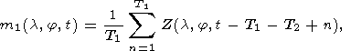
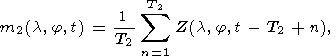
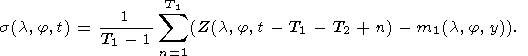
3.1. The procedure of data processing
The availability of spatially distributed synchronous observations allows one to
apply the space-time approach realized in the GEOTIME computer environment
[Gitis, et al., 1994; Gitis, et al., 1995].
The idea of this approach is based on the alternative of the method of data presentation.
The time variations of geophysical parameters synchronously measured at different points
of the region and the data of the earthquake catalogue are transformed into dynamic fields
representing three-dimensional rasters with two spatial and one temporal co-ordinates.
A sufficiently extensive set-up of space-time transformations over dynamic fields is
realized in the GEOTIME medium; these transformations allow us to generate various
secondary dynamic fields from the initial ones.
It is assumed that after elimination of seasonal rhythms in the absence of earthquake
preparation the dynamic fields are inhomogeneous in space, but quasistationary in time.
The appearance of a precursor, which occupies a certain related subset of elements of
the raster, violates the stationarity of the process.
In order to determine the non-stationarity, the current observation interval is
divided into two consecutive sub-intervals T1 and T2,
of which the former is several
times longer than the latter. The duration of both sub-intervals are determined by the
researcher depending on the statistical properties of the background signal within the
interval without precursor and on the expected duration of anomalous changes.
The problem is reduced to testing the hypothesis of statistical homogeneity of two
random sample sets. The hypothesis about the coincidence of parameters of the sample
set distributions is tested by a certain statistics, which depends on the selected
statistical model. In the case when several dynamic fields of different physical nature
are jointly analyzed (the multidisciplinary approach), their values at raster points
are multidimensional vectors, and multidimensional statistical models are used to verify
the hypothesis.
In our case, the vector dynamic fields, computed from the time series of different
types of the measured parameters, are not representative owing to the restricted number
of stations. We, therefore, resort to a compromise by using the GEOTIME system to obtain
a unified scalar dynamic field for all temporal series recorded at all available stations
regardless of the physical nature of the measured values.
For this purpose, the signals from all stations should be first of all standardized
(normalized by variances).
After standardization, the data processing is carried out by three stages, i.e.,
I - cleaning the time series of seasonal rhythms; II - calculation and transformation
of dynamic field of precursors; III - calculation and analysis of dynamic fields of
precursors' significance.
3.2. Stage I
In the course of the initial stage we proceeded from the generalized world
experience of research on earthquake prediction; its basic facts are that earthquake
precursors can be observed during several tens of years (long-term), several years and
several months (middle-term), weeks and days (short-term), and a few hours and less
(operative) before the moment of the actual earthquake.
The relatively short series of diurnal observations before the Tangshan and Datong
earthquakes of about 5 and 9 years duration, correspondingly, did not allow us to analyze
the long-term precursors, and we analyzed the possible appearance of only middle- and
short-term precursors. The rather large and complicated by form variations of seasonal
rhythms also provided little opportunity for identification of precursors with duration
of more than a year. Consequently, at the present state of research, the analysis was
aimed at finding anomalous changes of from one to several months duration.
The pattern of seasonal rhythm was estimated by the time series interval 2 years long.
It was assumed that the seasonal rhythm remains unchanged during the next year (the year of
prognosis). For example, the seasonal rhythm for the Tangshan earthquake was estimated by
data of 1972 and 1973 and predicted for 1974. This procedure was repeated for every
following year. In order to retain for analysis the whole observation series before
the Tangshan earthquake since 1972, the image of the seasonal rhythms, based on the
material of 1973-74 and 1974-75, was predicted backwards, i.e., for 1972 and 1973,
respectively. The seasonal patterns computed for all these years were then subtracted
from the initial time series.
Figure 1 (b, d)
shows examples of signals obtained after subtraction of seasonal
rhythms. It is obvious that these realizations contain not only anomalies associated
with incomplete removal of the seasonal trend, but also other deviations of unknown
nature and probably the earthquake precursors among them.
For different physical parameters the precursors can be both positive and negative
anomalies, as illustrated, in particular, by the given examples. In 1975-76, at one of
the stations, a lowering of the signal's level was recorded (Figure 1 (b)), whereas at
another station (Figure 1 (d)) the level has risen, and both anomalies can be regarded
as the possible precursors of the Tangshan earthquake.
3.3. Stage II
During stage II, the spatial interpolation is carried out for every time section of
signals from all stations. The signals were squared to avoid mutual exclusion during
interpolation of anomalies observed at different stations. For the dynamic field, the
raster was adopted having 0.1o in latitudinal direction, 0.067o
in meridian direction, and 5 days on the time coordinate. Interpolation was made by formula
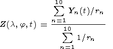 | (2) |
where Z(l, j, t)
is interpolated value at point (l, j, t),
Yn(t) is value of signal of n-station at
moment t, rn is the distance from n-station to the point
(l, j, t),
with rn = 0, Z(l,
j, t) = Yn(t).
3.4 Stage III
The third stage is aimed at identifying precursors in time and in space. With this
purpose in view, two statistical hypotheses were verified. The H0 hypothesis involves
mathematical expectations of sequences in the first window T1 and in the second window
T2Ha
hypothesis presumes that the mathematical
expectation of the sequence in the second window is greater than that in the first.
If Ha
hypothesis is applied, then it is assumed that a non-stationarity is observed
in T2 interval. If H0 hypothesis is selected,
then the process is recognized as stationary.
The verifying criterion of H0 hypothesis against
Ha
hypothesis is based on calculation of
statistics representing the difference of selected average values:
 | (3) |
where
T1 = 73, T2 = 6, which at 5-days step of the time co-ordinate corresponds to 365 and 30 days.
It is obvious that with H0 hypothesis the mathematical
expectation of statistics G(a, j, t)
is close to 0. But where as the counts down of the Z(a, j, t)
signal are strictly correlated, the
estimation of mean square deviations of the difference of selected averaged values,
if H0 hypothesis is applied, meets with great difficulties. Let us assume that with
H0 hypothesis the variance s2(a,
j, t) of the signal is a slowly varying function of t and so
it is the same in both windows T1 and T2. Then the upper
limit of the root mean square of random variable G(a, j, t)
is equal to 2s(a, j, t).
It is convenient to normalize the G statistics by
the statistical estimate of root mean square:
 | (4) |
where
The u(a, j, t)
statistics evaluates the degree of deviation from the stationary. With H0
hypothesis the statistics has the expectation close to 0 and the root mean square less
than 1.
Go to Contents
4.1. Tangshan
At selected duration of windows T1 and T2,
the period of 1972 is entirely reserved
to instructive material, and the first map of dynamic field of deviation statistics from
the stationary refers to January 1973. The maps that followed were compiled with the
5-days shift. In total, 257 maps were prepared for deviation analysis; the latest map
covers the period from June 24 to July 23, 1976.
The analysis of the maps reveal anomalies in July-August of some years owing to
incomplete removal of the seasonal rhythm. The periods from September through June are
free of this drawback, and their anomalies, apparently, had other causes including those
of geodynamic character.
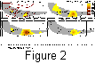 Unlike the two previous years, in September of 1975, a powerful anomaly with a
maximum occurred over almost the entire studied area of northeastern China. It gradually
attenuated and practically disappeared in April 1976. Only two anomalous stations remained,
TS and SQ, in the region of the future Tangshan earthquake. In May 1976, the anomaly in
the area of these stations grew intensively, as shown in
Figure 2 (1)
representing the
map of that period. At the same time, a less intensive anomaly appears in the Beijing
area. For easier orientation, Figure 2 (1)
also shows tectonic faults and epicenters of
the future Tangshan earthquake and of the two strongest aftershocks with magnitudes 6.9
and 7.0. There is a striking irregularity in the distribution over the territory of
recording stations that supplied the initial observation series.
Unlike the two previous years, in September of 1975, a powerful anomaly with a
maximum occurred over almost the entire studied area of northeastern China. It gradually
attenuated and practically disappeared in April 1976. Only two anomalous stations remained,
TS and SQ, in the region of the future Tangshan earthquake. In May 1976, the anomaly in
the area of these stations grew intensively, as shown in
Figure 2 (1)
representing the
map of that period. At the same time, a less intensive anomaly appears in the Beijing
area. For easier orientation, Figure 2 (1)
also shows tectonic faults and epicenters of
the future Tangshan earthquake and of the two strongest aftershocks with magnitudes 6.9
and 7.0. There is a striking irregularity in the distribution over the territory of
recording stations that supplied the initial observation series.
 The next map in Figure 2 (2)
represents the period from May 14 till June 13.
At that time the anomaly in the Beijing area reached its maximum, and that in Tangshan
was steadily growing. The map in Figure 2 (3)
(May 29-June 28, 1976) shows the maximum
of the anomaly in Tangshan region; after that time it gradually attenuates till the
moment of the earthquake (Figure 2 (4) ).
The dynamics of the development of anomalies
along the A-B profile of latitudinal strike (Figure 2 (4))
can be followed in Figure 3
.
The curves 1, 2, 3, 4 correspond to the periods of maps in
Figure 1 (1, 2, 3, 4).
The next map in Figure 2 (2)
represents the period from May 14 till June 13.
At that time the anomaly in the Beijing area reached its maximum, and that in Tangshan
was steadily growing. The map in Figure 2 (3)
(May 29-June 28, 1976) shows the maximum
of the anomaly in Tangshan region; after that time it gradually attenuates till the
moment of the earthquake (Figure 2 (4) ).
The dynamics of the development of anomalies
along the A-B profile of latitudinal strike (Figure 2 (4))
can be followed in Figure 3
.
The curves 1, 2, 3, 4 correspond to the periods of maps in
Figure 1 (1, 2, 3, 4).
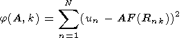
 For comparison, Figure 4
shows 6 maps of the previous three years covering the
period of the beginning (May 4-June 3) and the maximum (May 39-June 28) of the Tangshan
anomaly. It is apparent that during all these years, in the Tangshan area, no significant
anomalous changes were recorded in the field of the complex of studied parameters.
For comparison, Figure 4
shows 6 maps of the previous three years covering the
period of the beginning (May 4-June 3) and the maximum (May 39-June 28) of the Tangshan
anomaly. It is apparent that during all these years, in the Tangshan area, no significant
anomalous changes were recorded in the field of the complex of studied parameters.
4.2. Datong
A similar processing was carried out for the time series referring to the Datong
earthquake. In this case the first map of dynamic field of deviation statistics from the
stationary refers to January 1982. The maps that followed were compiled with the 5-days
shift. In total, 568 maps were prepared for deviation analysis; the latest map covers the
period from September 15 to October 14, 1989.
 An analysis of these maps shows that the dynamics of the field of the studied
parameters largely differ from the dynamics before the Tangshan earthquake. This is
evident from the series of maps in Figure 5.
During the period from July 21 till
August 20, 1989 (Figure 5a),
in the region of Tangshan, an anomaly appears, which
then grows in intensity and spreads west and east. The anomaly reaches its maximum
in the period from August 20 till September 19 (Figure 5c),
and then reduces (Figure 5d).
In this case, the irregularity of distribution of measurement stations becomes apparent.
In the southwest, there is only one TY station, and there are no data for the region of
the Datong earthquake.
An analysis of these maps shows that the dynamics of the field of the studied
parameters largely differ from the dynamics before the Tangshan earthquake. This is
evident from the series of maps in Figure 5.
During the period from July 21 till
August 20, 1989 (Figure 5a),
in the region of Tangshan, an anomaly appears, which
then grows in intensity and spreads west and east. The anomaly reaches its maximum
in the period from August 20 till September 19 (Figure 5c),
and then reduces (Figure 5d).
In this case, the irregularity of distribution of measurement stations becomes apparent.
In the southwest, there is only one TY station, and there are no data for the region of
the Datong earthquake.
 For comparison, a series of maps for the previous six years is demonstrated in
Figure 6
(1983-1988) for August - September; during that period in 1989, the anomaly
in the studied region reached its maximum. Apparently there no considerable anomalous
changes in intensity and area at that time.
For comparison, a series of maps for the previous six years is demonstrated in
Figure 6
(1983-1988) for August - September; during that period in 1989, the anomaly
in the studied region reached its maximum. Apparently there no considerable anomalous
changes in intensity and area at that time.
 The dynamics of the development of the anomaly in 1989 before the Datong earthquake
are shown in Figure 7.
The plots 1, 2, 3, 4 along the latitudinal profile A-B correspond
to the periods of corresponding maps in
Figure 5a, b, c, d.
The migration of the process
is clearly traced in the western direction; it is less distinct in the eastern direction
where the region is confined to the location of CL station. Unfortunately, the data of JX
station hear Haichen were not available to the anthars for the period of the Datong
earthquake.
The dynamics of the development of the anomaly in 1989 before the Datong earthquake
are shown in Figure 7.
The plots 1, 2, 3, 4 along the latitudinal profile A-B correspond
to the periods of corresponding maps in
Figure 5a, b, c, d.
The migration of the process
is clearly traced in the western direction; it is less distinct in the eastern direction
where the region is confined to the location of CL station. Unfortunately, the data of JX
station hear Haichen were not available to the anthars for the period of the Datong
earthquake.
4.3. Modelling of epicentral anomalies
4.3.1. Justification of the model
A comparison of dynamic fields (Figure 2
and Figure 5)
shows that the shape and
size of the anomaly that precedes the Tangshan earthquake greatly differs from the
anomaly before the Datong earthquake. The Tangshan anomaly almost covers the region
of the future epicentral earthquake zone, while the Datong anomaly covers practically
the whole area on which the stations are located. We can suppose that these anomalies
reflect different mechanisms of manifestation of precursors. The Tangshan anomaly shows
that the generation of precursors has local character and is connected with the focus
of the expected earthquake. But the Datong anomaly demonstrates the regional character
of earthquake preparation, where precursors have on indirect association with the focus
through the changes of tectonic stresses on a vast territory.
The epicentral character of manifestation of precursors was discussed in
[Chen Yong, et al., 1992; Zhang Zhaocheng,
et al., 1992], where retrospective data are given on the dependence between
the relative number of stations that recorded the precursor and the distance to the
earthquakes epicenters. For the earthquakes with magnitude 7, these data are
given in Table 2.
Let us assume that at distances of the order of 1000 km, the precursors cease to
bee observed and the amplitude of a precursor diminishes approximately by the same law
as the number of stations that recorded the earthquake precursors. In this case,
Table 2
can be approximated by the attenuation function
| F(R) = A(exp(-0.02R) - 0.27) | (5) |
where A is the amplitude of the signal, R is the distance to the source of the signal
in km.
In this part of the paper we shall make an attempt to model a generalized precursor
of the Tangshan earthquake by using the attenuation model (5) to localize the future source.
Let us indicate the time series obtained on observation stations n = 1, 2, ..., N
by u(n, t). We shall assume that, for any fixed moment of time, the center of the
precursor's signal coincides with one of the points of the raster k = 1, 2, ..., K
and that the values of the time series at the observation stations are expressed by
relationship
where A is the amplitude of the signal, k is the number of the raster point,
in which the center of the signal is located; xn
are the independent Gauss values with zero
mathematical expectancy and the mean square deviation s.
4.3.2. Estimation algoritm
Let us estimate the parameters of the signal by the method of least squares.
The estimations are obtained by minimizing the functional
 | (7) |
With known k =  and if the signal propagates from point ,
the estimation of the amplitude A()
is determined by expression
and if the signal propagates from point ,
the estimation of the amplitude A()
is determined by expression
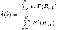 | (8) |
By sorting out all the possible values of k = 1, 2, ..., K, we obtain different
values of A() and residual sums
of squares
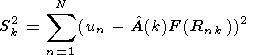 | (9) |
In order to evaluate the center of the signal - the K point-, let us analyse the
criterion of relation of square estimation of the measured signal to the square of
discrepancy (signal/noise ratio)
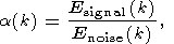 | (10) |
where
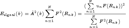 | (11) |
We should note that the vectors of the signal
F = (F(R1k), F(R2k), . . . ,
F(Rnk)) and of the discrepancy, obtained by the least squares
method, are orthogonal and in sum compose the vector of observations
u = (u1, u2, . . . , uN).
Therefore,
 | (12) |
and
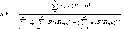 | (13) |
If we suppose that at the analysed moment of time the signal is absent, that is
un = xn,
then a(k) is the relation of the Gauss square
value with zero mathematical expectancy and dispersion s2
to the sum of squares N-1 of Gauss values with the same parameters.
It is convenient, instead of a(k), to consider
the monotonously associated with it value
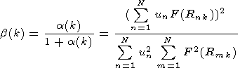 | (14) |
Value b(k) acquires the magnitude ranging from 0 to 1.
The value b(k) = 1 corresponds
to the situation when un = AkF(Rnk),
i.e., the signal/noise ratio is equal to  .
At b(k) = 0, the
signal is absent. At b(k)
.
At b(k) = 0, the
signal is absent. At b(k)  0.5,
the discrepancy in parameter A evaluation is greater
than the amplitude evaluation. Therefore, independently of the value of amplitude
Ak estimation, we can admit that, in the studied region, the signal corresponding to the
assumed model was not observed.
0.5,
the discrepancy in parameter A evaluation is greater
than the amplitude evaluation. Therefore, independently of the value of amplitude
Ak estimation, we can admit that, in the studied region, the signal corresponding to the
assumed model was not observed.
On the basis of these considerations, at b(k) 0.5,
the estimation of the position of the signal
center we shall choose for the condition of the maximum of function b(k),
k = 1, 2,..., K, i.e.,
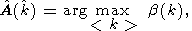 | (15) |
and  ()
value shall be assumed as the estimation of the amplitude of the signal.
()
value shall be assumed as the estimation of the amplitude of the signal.
4.3.3. Modelling
The modelling of the epicentral anomaly of the Tangshan earthquake was carried out
on the basis of the average diurnal time series obtained at stations 1 to 10
(Table 1).
It was presumed that the Tangshan earthquake precursours are generated by one source
located within the polygon (Figure 2),
and the change of the signal is described by
equation (5).
The first stage of processing, as in part 3, included standartization of series,
suppression of the seasonal rhythms, and squaring. At the next stage, the time series
of deviations for stationarity were calculated by formulas (3) and (4) with substitution
in them of coordinates l, j
by the number of the stations is at the value of parameter
T1 = 365 days and T2 = 30 days.
The last stage was the transition to the space-time model
by estimation of parameters of the model
and ()
with 5 days interval.
Figure 7
shows plots of changes of criterion of the presence of signal
b(),
estimation of its amplitude ()
and the distance r(, C)
between the center of signal
and the real earthquake epicenter. It is apparent that during almost the whole
interval up to August 1975 b() < 0.5.
This means that, according to our supposition,
the epicentral precursor signal was either absent, or did not comply to the model (5).
A year before the earthquake, since August-September 1975, the b()
values sharply increased and exceeded 0.5. In other words, at that time interval, the suggested
model conforms best with the set of real data. Concurrently, an essential increase
of the signal's amplitude was recorded. Finally, since November 1975, the center of
the modelled anomaly was shifted to the epicentral area of the Tangshan earthquake
with deviations from the future epicenter reaching about 50 km.
Go to Contents
The present paper suggests a new technology of space-time analysis of geophysical
series tested by real data. The study is based on transition from the analysis of time
series to the analysis of trivariate rasters - with two spatial and one temporal coordinates.
Two approaches were realized:
- spatial interpolation of observation data and compilation of time sections;
- calculation from time sections of spatial anomalies according to a certain hypothesis about the geometry of the precursor.
The following preliminary conclusions can be drawn from the analysis of
the initial data and maps at our disposal showing the complex of the studied
geophysical, hydrogeological and geochemical parameters.
From May till July 1976, an anomaly was recorded in the region of the
future Tangshan earthquake; its amplitude, probably, exceeded the random
deviations of the background noise. The coincidence of the maximum of the
anomaly with the Tangshan earthquake and the absence of such anomaly in the
analyzed previous years does not contradict the hypothesis about its geotectonic origin.
If that supposition is true, then the anomaly is a medium-short -term precursor
that appeared in the vicinity of the earthquake's focus. Let us recall that precursors
with duration longer than a year or less than a few days are not analyzed in this paper
on account of restricted observation series.
On the other hand, the Datong earthquake of October 19, 1989, occurred against the
background of regional anomaly covering a large part of north-eastern China and localized
near the epicenter. We believe, that the earthquake proper is only indirectly connected
with the observed anomaly in the field of geophysical parameters. Both events could have
been caused by regional changes in the stress state of the environment the nature of
which is as yet unknown.
We wish to emphasize that our conclusion is open to further revision, because it is
based on obviously incomplete experimental data and extremely irregular observation network.
Other conclusions of the present research are as follows.
It is necessary to eliminate all possible errors of external origin in the initial data.
It is desirable to add to the analysis the available observation series from a larger
set of stations preferably covering the area with greater regularity.
It seems expedient to carry out a formalized comparison of the available series of
prognostic observations with similar series of certain meteorological parameters and,
primarily, the air and soil temperature, the amounts of precipitation, and atmospheric
pressure.
It is important to include into the processing the data on seismicity for better
insight into the geodynamic process.
The prognostic features could be more readily identified by creation of models of
space-time precursors formation based on the physics of the earthquake focus and on the
experience of experimental observations.
Meanwhile, the elaborated variant of the GEOTIME system allows us to study the
geodynamic process using a complex of heterogeneous data of prognostic observations.
The experience of the present research has indicated the direction in which further
development of the system should be continued.
Go to Contents
We extend our thanks to the collaborators at the Center for Analysis and Prediction,
SSB, China, who have kindly made available the materials of experimental observations.
The work was accomplished within the frame of the Agreement between the State Seismological
Bureau of China and the Russian Academy of Sciences.
The research is supported by grants No. 97-05-65906 and No. 97-07-90326 from Russian
Foundation for Basic Researches.
Go to Contents
1. Ma Zonglin, Fu Zhengxiang, Zhang Yingzhen et al., Earthquake Prediction. Seismol. Press:
Springer, 1989, p.332.
2. Continental Earhquakes. Seismol. Press, Beijing, 1993, p. 576.
3. Sobolev G. A., Fundamentals of Earthquake Prediction. Nauka, Moscow, 1993, p. 311
(in Russian).
4. Gitis V. G., Osher B. V., Pirogov S. A., Ponomarev A. V. , Sobolev G. A., Jurkov E. F.,
A System for Analysis of Geological Catastrophe Precursors. Journal of Earthquake
Prediction Research, Vol. 3, no. 4, 1994, pp. 540-555.
5. Gitis V. G., Osher B. V., Pirogov S. A., Ponomarev A. V. , Sobolev G. A., Jurkov E. F.,
Dynamic Fields Analysis System. Cahiers du Centre Europeen de Geodynamique et de
Seismologie, Vol. 9, 1995, pp. 129-140.
6. Chen Yong,Wang Wei, Zhu Yueqing and Ji Ying., Multidisciplinary approach used in
expert system for earthquake prediction in China. Journal of Earthquake Prediction
Research, Vol. 1, no. 1, 1992, pp. 107-113.
7. Zhang Zhaocheng, Zheng Dalin, Luo Yongsheng and Jia Qing., Studies on earthquake
precursors and the multidisciplinary earthquake prediction in China mainland.
Journal of Earthquake Prediction Research, Vol. 1, no. 2, 1992, pp. 191-205.
Go to Contents
HTML version prepared and loaded by
V. Nechitailenko on September 29, 1997
Go to Content of GPO, No. 1