
RUSSIAN JOURNAL OF EARTH SCIENCES, VOL. 20, ES4003, doi:10.2205/2020ES000731, 2020
Marek Stastna, Kevin G. Lamb
Department of Applied Mathematics, University of Waterloo, Ontario, Canada
In the theory of internal waves in the coastal ocean, linear stratification plays an exceptional role. This is because the nonlinearity coefficient in KdV theory vanishes, and in the case of large amplitude waves, the DJL theory linearizes and fails to give solitary wave solutions. We consider small, physically consistent perturbations of a linearly stratified fluid that would result from a localized mixing near a particular depth. We demonstrate that the DJL equation does yield exact internal solitary waves in this case. These waves are long due to the weak nonlinearity, and we explore how this weak nonlinearity manifests during shoaling.
Internal waves are an important physical phenomenon in the world's oceans primarily because of their role in cascading energy from large to small scales where they break, dissipate and mix. The two primary generation mechanisms for internal waves are tide-topography interactions and wind stress at the ocean surface, each contributing approximately half of the energy in the oceanic internal wave field [Waterhouse et al., 2014]. Internal waves have several interesting properties. The frequency of a linear internal plane waves is a function of the direction of its wave vector in the vertical plane which has several far reaching consequences. For example wave energy propagates along wave crests rather than in the direction of phase propagation and waves reflect off a bottom slope with their angle to the vertical preserved rather than their angle to the boundary (i.e. Snell's law). One consequence of the latter is wave focusing after upslope reflection which increases wave energy density and transfers energy to shorter wavelengths.
Another interesting internal wave phenomenon are internal solitary-like waves (ISWs) which are ubiquitous in coastal regions of the world's oceans where they predominantly form via the nonlinear-dispersive evolution of internal tides (internal waves of tidal frequency generated by tide-topography interaction) [Jackson et al., 2012]. These waves propagate horizontally in the wave guide bounded by the surface and bottom. For a continuously stratified fluid there are a discrete set of modes which have different vertical structures. By far the most commonly observed and most energetic ISWs are mode-one waves. Mode-one waves are characterized by having isopycnals which are all vertically displaced in the same direction: downward for waves of depression and upward for waves of elevation. Mode-two waves are observed less frequently [Shroyer et al., 2010a; Liang, 2019]. They have ispopycnal displacements in one direction in the upper part of the water column and in the opposite direction in the lower part and propagate much more slowly. In general the direction of isopycnal displacements changes sign $n-1$ times in a mode-$n$ wave.
Fully nonlinear internal solitary waves can be modeled with the Dubreil-Jacotin-Long (DJL) equation [Turkington et al., 1991; Lamb and Wan, 1998; Stastna and Lamb, 2002]. This equation has the appealing feature that it can model fully nonlinear-dispersive waves however as it can only model mode-one waves of permanent form it can not be used to investigate the interaction of nonlinear internal waves or their evolution as they propagate through a changing environment, e.g. a region with variable water depth or currents. Long weakly-nonlinear ISWs and other long weakly-nonlinear horizontally propagating waves such as internal bores can be modeled with the well-known Korteweg-de Vries (KdV) equation
\begin{equation} \tag*{(1)} B_t + c_0B_x + \alpha BB_x + \beta B_{xxx} = 0 \end{equation}which does enable investigations of an evolving wave field including shoaling waves after the addition of a shoaling term [Grimshaw et al. 2004; Lamb and Xiao, 2014]. This equation has solitary wave solutions which have an number of fascinating properties. They are waves of permanent form with a very particular shape that arises through a balance of nonlinear and dispersive effects. As their amplitude increases they get narrower and their propagation speed increases. Two solitary waves of different amplitude can therefor interact when a large wave catches up to a smaller wave and after a complicated nonlinear interact the two waves re-emerge with exactly the same amplitudes and shape that they started with, leading to the name `soliton' for waves with this special property. Solitary waves solutions of the KdV equation are waves of depression if $\alpha<0$ and waves of elevation if $\alpha>0$.
In the ocean internal waves are often large enough to necessitate the inclusion of higher-order nonlinearity in weakly-nonlinear models which leads to the Gardner equation
\begin{equation} \tag*{(2)} B_t + c_0B_x + \alpha B B_x + \alpha_1B^2 B_x + \beta B_{xxx} = 0. \end{equation}Further extensions are possible [Pelinovskii et al., 2000]. While extending the range of validity of the KdV equation the Gardner equation also has some new features. Of some significance is that the cubic coefficient $\alpha_1$ can have either sign in the ocean [Grimshaw et al., 1997; Grimshaw et al., 2007]. If $\alpha_1<0$ solitary waves now have a maximum amplitude and become broad and flat-crested as this limiting amplitude is approached, a feature of fully nonlinear internal solitary waves. Such waves have occasionally been observed in the field [Shroyer et al., 2010b]. The case when $\alpha_1>0$ is particularly interesting: solitary waves of either polarity (i.e. waves of depression and waves of elevation) can now exist and a new type of nonlinear wave, a pulsating packet called a breather, exists [Grimshaw et al., 2007].
Because of the rich nonlinear-dispersive behavior of internal waves they have been a topic of research for decades. For a linear stratification under the Boussinesq approximation both nonlinear coefficients of the Gardner equation are zero and the DJL equation, used to model fully nonlinear ISWs, linearizes and has no solitary wave solutions. Small perturbations to a linear stratification reintroduce nonlinearity albeit very weakly. In this manuscript we explore a few curious features of these waves which, while perhaps not physically relevant to the ocean, never-the-less enrich our understanding of these fascinating waves.
Useful theoretical and computational tools for studying ISWs in the ocean include weakly-nonlinear theories, the DJL equation and fully nonlinear numerical models. The latter can be computationally expensive because of the necessity of including non-hydrostatic effects and the high resolution required to resolve the waves coupled with often large domains when studying their shoaling behaviour [Lamb et al., 2015]. Weakly-nonlinear models have the advantage of being quick making it easier to more fully explore parameter space and to focus on some key processes [Holloway et al., 1999; Grimshaw et al., 2007; Grimshaw et al., 2010; Lamb and Xiao, 2014].
The second order finite volume code, IGW solves the 2D, nonlinear, non-hydrostatic, Boussinesq equations [Lamb, 2007]. The version of the model equations solved here ignore rotational and viscous effects and are
\begin{eqnarray*} \Bigl(\vec{u}_t + \vec{u}\cdot\vec{\nabla}\vec{u}\Bigr) &= -\vec{\nabla} p - \rho g \hat{k} \end{eqnarray*} \begin{eqnarray*} \rho_t + \vec{u}\cdot\vec{\nabla}\rho &= 0 \end{eqnarray*} \begin{eqnarray*} \vec{\nabla}\cdot\vec{u} &= 0, \end{eqnarray*}where the 2D velocity in the $xz$-plane is $\vec{u} = (u,w)$, represented by the $\hat{i}$ and $\hat{k}$ unit vectors respectively. The dimensionless density $\rho$ represents the variations in the density about the reference density $\rho_0$, so the physical density is $\rho^* = \rho_0(1+\rho)$. The pressure $p$ is the difference between the physical density $p^*$ and the pressure in hydrostatic balance with the reference density and has also been scaled by $\rho_0$. No variation occurs in the $y$ direction (i.e. $\partial / \partial y = 0$) maintaining the 2D approach. The model uses a second-order, finite volume projection method [Bell et al., 1989; Bell and Marcus, 1992].
The model has a rigid lid and uses terrain following coordinates thus increasing the resolution over the shelf. We used 200 grid points in the vertical (i.e. a resolution of $0.75$ m) with a horizontal resolution of 12 m.
Weakly nonlinear theories (WNL) of internal wave motion start with the stratified incompressible Euler Equations, shown above under the Boussinesq approximation and in the absence of rotation. We assume a flat ocean bottom located at $z=-H$. WNL performs an expansion of these equations in two parameters, one that specifies a small but finite amplitude, and the other that specifies a small aspect ratio, or ratio of typical vertical to typical horizontal length scales. For example, in the $xz$-plane, when written in terms of the isopycnal displacement $\eta(x,z,t)$ WNL assumes
\begin{eqnarray*} \eta(x,z,t)=B(x,t) Z(z) \end{eqnarray*}at leading order. A systematic perturbation expansion then derives an eigenvalue problem for $Z(z)$,
\begin{eqnarray} Z" + \frac{N^2}{c^2}Z &= 0, \nonumber Z(-H) = Z(0) &= 0. \nonumber \end{eqnarray}Here
\begin{eqnarray*} N^2(z) = - g \bar{\rho}'(z) \end{eqnarray*}where $\bar{\rho}(z)$ is the background density profile. Continuing to the next order in amplitude and aspect ration, the perturbation expansion also yields an evolution equation for the wave form $B(x,t)$, e.g. the KdV equation (1). The nonlinear and dispersive coefficients of the KdV equation are given by
\begin{eqnarray*} \alpha &= {3c\over2}{\int_{-H}^0Z'^3\,dz\over \int_{-H}^0Z'^2\,dz} \end{eqnarray*} \begin{eqnarray*} \beta &= {c\over2}{\int_{-H}^0Z^2\,dz\over \int_{-H}^0Z'^2\,dz}. \end{eqnarray*}The Dubreil-Jacotin Long (DJL) equation is formally equivalent to the full set of stratified Euler equations [Turkington et al., 1991; Lamb and Wan, 1998; Stastna and Lamb, 2002]. Its solutions thus describe exact internal solitary waves. In a frame moving with the solitary wave, the DJL equation under the Boussinesq approximation reads
\begin{eqnarray*} \nabla^2 \eta + \frac{N^2(z-\eta)}{c^2}\eta = 0 \end{eqnarray*}with homogeneous (i.e. $\eta=0$) boundary conditions at $z=-H,0$ and as $|x|\rightarrow \infty$. When $N^2=N_0^2$ is constant, or in other words when the density profile is linear, the DJL equation linearizes. In this case standard theory of linear elliptic equations shows that the maximum of $\eta$ must occur on the boundary and solitary waves are thus impossible.
We consider density profiles of the form
\begin{eqnarray*} {\bar{\rho}(z)} = -\Delta \rho \frac{z}{H}+a_p \tanh\left(\frac{z-z_0}{d}\right)\textrm{sech} \left(\frac{z-z_0}{d}\right) \end{eqnarray*} |
| Figure 1 |
(see Figure 1). Here $\Delta \rho$ specifies the top to bottom density change for the linear stratification, while the second term models a mixed layer centered at $z_0$ with a thickness characterized by $d$. We choose $\Delta \rho=0.01$, or a $1\%$ density change from domain top to bottom. $a_p$ sets the amplitude of the perturbation, which has a functional form chosen so that integral of the perturbation is zero. The centre of the perturbation consists of less stratified (i.e. partially mixed) fluid, while the flanks of the perturbation are more strongly stratified. In practice $a_p$ must be quite small, in order to preclude local density overturns. While we varied $a_p$, results reported below fix $a_p=0.0002$. We will vary $z_0$, but fix $d=0.025 H$.
 |
| Figure 2 |
We considered the effect of the density perturbation on the first 10 modes of linear theory as a function of depth. We define $c_{base}$ as the solution for the linear stratification, and compute the relative error. For vertical structure functions we compute the $L^2$ difference between the mode in the perturbed case and the mode in the linear stratification case. The results are summarized in Figure 2. The top row shows the results for all 10 modes. It is readily apparent that higher modes are more strongly affected by the perturbation. The perturbation form is schematized in the lower left panel, where $N^2$ is shown. Since the effects on the lower modes were difficult to see when all modes were shown, the lower right panel shows the $L^2$ difference for the first three modes. It is apparent again, that the effect on the lowest mode is very small compared to that on the higher modes. This is what motivated us to look at the DJL equation next, to see if a qualitative difference for mode-1 could be observed.
Solutions of the DJL equation were computed by the variational method due to Turkington and co-workers [Turkington et al., 1991] as implemented in [Lamb and Wan, 1998; Stastna and Lamb, 2002]. Due to the weak nonlinearity the convergence of the iteration procedure was considerably slower than in stratifications with much larger variations in the buoyancy frequency that are more typical for the ocean.
 |
| Figure 3 |
Figure 3 shows the density field for four sample internal solitary waves, two (panels a and b) for a mixed layer centered at $z_0 = -25$ m and two (panels c and d) for a mixed layer centered at $z_0 = -15$ m. The location of the center of the mixed layer is indicated by a dashed black line. It is immediately clear that changing the mixed layer location can lead to a change in solitary wave polarity. The waves of elevation have a fairly generic, bell-like shape, while the waves of depression are quite a bit broader.
 |
| Figure 4 |
Figure 4 shows bulk wave properties as functions of the available potential energy, $APE$, for the waves of elevation (the mixed layer centered at $z_0=-25$ m). Panel (a) shows the maximum isopycnal displacement, panel (b) shows the propagation speed, panel (c) the wave half-width, and panel (d) shows some sample surface currents for a range of wave amplitudes It is clear that as the $APE$ increases the wave amplitude and propagation speed gradually increase, approaching the conjugate flow values [Lamb and Wan, 1998], while the half-width initially decreases as predicted by KdV theory before increasing as the waves broaden. The broadening of the waves is evident in the surface current plot. The extremely weak nonlinearity leads to only very small changes in propagation speed as the wave amplitude increases. It is also responsible for the very long lengths of the waves: the wave nonlinearity is balanced by dispersion which is very weak for long waves. This will be seen to have implications for wave behavior when shoaling. The gradient Richardson number (not shown) remains large in all cases, implying that shear instability will not play a role in the evolution of these waves.
 |
| Figure 5 |
Figure 5 shows the corresponding information for the waves of depression when the mixed layer is centered at $z_0 = -10$ m.
It is evident from Figure 3 that a small change in the height of the perturbation has led to a change in wave polarity. Indeed the waves with the smaller $z_0$ are even broader than those in the base case as is predicted by the much smaller magnitude of $\alpha$ for this stratification. The questions is, thus, in an ocean setting where a wave of depression shoals onto a shelf, is the nonlinearity strong enough for a reversal of polarity to be observed? And if the answer to this question is `No', then how is nonlinearity manifested?
 |
| Figure 6 |
Given the weak nonlinearity of the perturbed linear stratification and the observation that perturbations at different heights yield different polarities of internal solitary waves, we wanted to assess how large amplitude internal waves evolve during shoaling. The stratification used is the stratification used for the ISWs shown in Figure 6. Figure 6a shows the shape of the bathymetry which was chosen so that the mixed layer is at depths of 15% and 25% of the water depth in the deep and shallow water corresponding to the depths of the mixed layer in the example waves in Figure 3. The remaining panels show the initial wave–induced surface (solid line) and bottom (dashed line) horizontal velocity profiles (panel (a)); and the wave–induced surface (solid line) and bottom (dashed line) horizontal velocity profiles after shoaling (panel (b)). The reader should note the extremely long length scale of the initial wave which is based on KdV theory, i.e. it is not a DJL solution. In spite of this is propagates without noticeably changing shape until it shoals onto the shelf.
It is immediately evident that the shoaling process leads to both an asymmetry in the horizontal structure and significant shedding of waves behind the leading wave. The back of the wave is quite steep (though recall that this wave is very long and hence the wave is not close to breaking). On the scale of the figure only a mode-1 tail is evident. Higher mode waves are found further behind the leading wave, and will be discussed below. It is interesting that the long tail is accompanied by a train of short length scale waves. On the scale of the figure these are difficult to see as anything more than `squiggles', but they are well-resolved by the numerical model with at least twenty grid points per wavelength.
 |
| Figure 7 |
In Figure 7 we show the horizontal velocity field (shaded) and density field (black) associated with the mode-1 wave after it has moved onto the shelf. The horizontal asymmetry of the wave is evident in both the horizontal velocity and density fields, while evidence of short wave generation is found not only at the back of the wave, but in weaker form near the front of the wave. The fact that short wave activity is possible near the front is due to the extremely weak nonlinearity of the system. In other words the mode-1 wave cannot outrun the shorter waves on the timescales shown.
 |
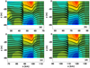
| Figure 8 |
In Figure 8 we show the horizontal velocity field (shaded) and density field (black) associated with the trailing, higher mode waves after the main wave has moved onto the shelf. In panel (a) the trailing face of the leading wave is visible near the right of the figure. The evolution is clearly dominated by a long mode-2 wave which maintains its form for all times shown. This wave is not exactly horizontally symmetric across its crest, but its asymmetry is far less prominent than that of the leading mode-1 wave. At the back of the mode-2 wave several rapid horizontal transitions are observed. The authors are not aware of any article that reports such sharp transitions and they appear to be a novel manifestation of nonlinear behavior in this parameter regime.
 |
| Figure 9 |
The details of the shoaling process are shown in Figure 9. The leading wave steepens at the back and a mode-2 wave can be seen to be generated behind the leading wave as the leading wave reaches the on-shelf portion of the domain. Had we not identified the stratification as exceptional for the reader, it would be difficult to identify how this portion of the evolution differs from that in a linearly stratified fluid.
We have presented results on internal waves for stratifications that are `close to' a linearly stratified fluid; a case that is known to be exceptionally weak in terms of nonlinearity. The perturbations were representations of a local mixing event, in that the mean perturbation was zero with some regions with a reduced buoyancy frequency and some with an increased buoyancy frequency.
Linear theory suggested that higher mode waves are more strongly affected than lower mode waves, but that even mode-1 waves had some changes in the vertical structure. For exact solitary waves, the DJL equation has no solutions in the linearly stratified case, and the perturbations did allow for solutions to be found. However, the weak nonlinearity meant that convergence of the iterative algorithm was slow, and the resulting waves were very long. Somewhat surprisingly, small changes in the perturbation location led to a change of solitary wave polarity and this motivated us to consider shoaling of such waves.
Numerical experiments suggest that the shoaling waves do not have time to form a clear undular bore, or wave train of solitary waves of the opposite polarity. Instead, the leading mode-1 wave develops short length scales on its trailing slope. Small perturbations are also observed on the leading slope. These are possible due to the extremely small range of variations in propagation speeds in the solutions of the DJL equations. Much stronger nonlinear effects are observed in the higher mode waves that trail the leading mode-1 wave. Here a prominent, long mode-2 wave is trailed by sharp transitions in the density field.
Future work could consider the weakly nonlinear description of the shoaling process to answer the theoretical question of whether a true reversal of polarity and the formation of a well defined wave train takes place. An obvious avenue for numerical simulations would involve consideration of higher modes and the sharp fronts they exhibit on the shelf.
Bell, J. B., D. L. Marcus (1992) , A second-order projection method for variable-density flows, J. Comp. Phys., 101, no. 2, p. 334–348, https://doi.org/10.1016/0021-9991(92)90011-M.
Bell, J. B., P. Colella, H. M. Glaz (1989) , A second-order projection method for the incompressible navier-stokes equations, J. Comp. Phys., 283, no. 85, p. 257–283, https://doi.org/10.1016/0021-9991(89)90151-4.
Grimshaw, R., E. Pelinovsky, T. Talipova (1997) , The modified Korteweg-de Vries equation in the theory of large-amplitude internal waves, Nonlinear Processes in Geophysics, 4, p. 237–250, https://doi.org/10.5194/npg-4-237-1997.
Grimshaw, R., E. Pelinovsky, T. Talipova (2007) , Modelling Internal Solitary Waves in the Coastal Ocean, Surv. Geophys., 28, no. 4, p. 273–2981, https://doi.org/10.1007/s10712-007-9020-0.
Grimshaw, R., E. Pelinovsky, et al. (2004) , Simulation of the Transformation of Internal Solitary Waves on Oceanic Shelves, J. Phys. Oceanogr., 34, no. 12, p. 2774–2791, https://doi.org/10.1175/JPO2652.1.
Grimshaw, R., E. Pelinovsky, et al. (2010) , Internal solitary waves: propagation, deformation and disintegration, Nonlin. Processes Geophys., 17, p. 633–649, https://doi.org/10.5194/npg-17-633-2010.
Holloway, P. E., E. N. Pelinovsky, T. G. Talipova (1999) , A generalized Korteweg-de Vries model of internal tide transformation in the coastal zone, J. Geophys. Res., 104, p. 18,333–18,350, https://doi.org/10.1029/1999JC900144.
Jackson, C. R., J. C. B. Da Silva, G. Jeans (2012) , The generation of nonlinear internal waves, Oceanography, 25, no. 2, p. 108–123, https://doi.org/10.5670/oceanog.2012.46.
Lamb, K. G. (2007) , Energy and pseudoenergy flux in the internal wave field generated by tidal flow over topography, Cont. Shelf Res., 27, p. 1208–1232, https://doi.org/10.1016/j.csr.2007.01.020.
Lamb, K. G., B. Wan (1998) , Conjugate flows and flat solitary waves for a continuously stratified fluid, Phys. Fluids, 10, p. 2061–2079, https://doi.org/10.1063/1.869721.
Lamb, K. G., A. Warn-Varnas (2015) , Two-dimensional numerical simulations of shoaling internal solitary waves at the ASIAEX site in the South China Sea, Nonlin. Processes Geophys., 22, p. 289–312, https://doi.org/10.5194/npg-22-289-2015.
Lamb, K. G., W. Xiao (2014) , Internal solitary waves shoaling onto a shelf: Comparisons of weakly-nonlinear and fully nonlinear models for hyperbolic-tangent stratifications, Ocean Modelling, 78, p. 17–34, https://doi.org/10.1016/j.ocemod.2014.02.005.
Liang, J., X.-M. Li (2019) , Generation of second-mode internal solitary waves during winter in the northern South China Sea, Ocean Dyn., 69, p. 313–321, https://doi.org/10.1007/s10236-019-01246-6.
Pelinovsky, E. N., O. E. Polukhina, K. Lamb (2000) , Nonlinear Internal Waves in the Ocean Stratified in Density and Current, Oceanol, 40, no. 6, p. 757–766.
Shroyer, E. L., J. N. Moum, J. D. Nash (2010a) , Mode 2 waves on the continental shelf: Ephemeral components of the nonlinear internal wavefield, J. Geophys. Res., 115, p. C07001, https://doi.org/10.1029/2009JC005605.
Shroyer, E. L., J. N. Moum, J. D. Nash (2010b) , Energy transformations and dissipation of nonlinear internal waves over New Jersey's continental shelf, Nonlin. Processes Geophys., 17, p. 345–360, https://doi.org/10.5194/npg-17-345-2010.
Received 7 October 2019; accepted 18 December 2019; published 12 July 2020.

Citation: Stastna Marek, Kevin G. Lamb (2020), An interesting oddity in the theory of large amplitude internal solitary waves, Russ. J. Earth Sci., 20, ES4003, doi:10.2205/2020ES000731.
Copyright 2020 by the Geophysical Center RAS.