
RUSSIAN JOURNAL OF EARTH SCIENCES, VOL. 19, ES4006, doi:10.2205/2019ES000672, 2019
Victor Zhurbas1, Germo Väli2, Andrey Kostianoy1,3, Olga Lavrova4
1Shirshov Institute of Oceanology RAS, Moscow, Russia
2Tallinn University of Technology, Department of Marine Systems, Tallinn, Estonia
3S. Yu. Witte Moscow University, Moscow, Russia
4Space Research Institute RAS, Moscow, Russia
An ultra-high resolution circulation model (0.125 nautical mile grid) of the Southeastern Baltic Sea is compiled from the General Estuarine Transport Model (GETM) in order to simulate the mesoscale eddy field in the area. The model results are compared with optical and infrared satellite imagery available for the period of May–August 2015. Mesoscale eddies detected in the satellite images are reasonably well identified in the simulated patterns of the sea surface temperature, currents, and floating Lagrangian particles.
The baroclinic Rossby radius of deformation, $R_{BC}$, is the basic length scale for the size of mesoscale eddies, which determine the weather in both the atmosphere and ocean. A typical value of $R_{BC}$ for the troposphere is $R_{BC} =1000$ km, and the number of sites of quasi-simultaneous (e.g., daily) measurements of meteorological parameters in a $R_{BC} \times R_{BC}$ square, $n$ is sufficiently large $(n \gg 1)$ to construct a weather map. According to recent data, there is one land-based meteorological station for every 1500 km$^2$ on the average [Kostianoy, 2017], i.e., $n=667$. The weather maps/data from yesterday and today can be extrapolated for tomorrow (or, more sophistically, assimilated in atmospheric models), which is a straightforward approach to the weather forecast. A typical value of the baroclinic Rossby radius in the ocean is much smaller than in the atmosphere, namely, $R_{BC}=30$ km in the middle latitudes, so that basically the number of oceanographic measurements in a $R_{BC} \times R_{BC}$ square is much smaller than one, and thousand times more oceanographic measurement sites per unit square are needed to resolve the ocean weather map to the same degree of detail as the weather map in the atmosphere. Note that the most advanced ocean-observing program Argo consisting currently of 3988 (as of 24 November 2018) free-drifting profiling floats in the World Ocean (see http://www.argo.ucsd.edu/) provides only one float in a $94 \times R_{BC} \times R_{BC}$ square or $n \approx 0.011$, which is far from being enough to construct the ocean weather map. Nevertheless, further progress towards the ocean weather forecast is believed to be achieved by using numerical modeling and remote sensing technologies, such as, e.g., Argo drifters and satellite altimetry [Vignudelli et al., 2011].
|
| Figure 1 |
However, the mesoscale ocean dynamics forecast (i.e., the weather) in relatively shallow inland/coastal seas, where the circulation strongly depends on the wind direction and strength, as well as on the coastline configuration and bottom topography, such as the Baltic Sea, is less challenging than in the open ocean because the process of forming of mesoscale eddies and fronts here becomes predictable to a certain extent. Thus, for example, it is known that in the case of an alongshore wind favorable for coastal upwelling frequently observed in the Baltic Sea [Lehmann and Myrberg, 2008; Myrberg and Andrejev, 2003], cyclonic eddies are formed behind the topographic features of the coastline (headlands or capes) and bottom elevations; these eddies can eventually break away from the formation sites and travel into the open sea (e.g. [Elkin and Zatsepin, 2013; Ginzburg et al., 1998; Zhurbas et al., 2017]). Moreover, not only the place of probable formation of a cyclonic vortex is known, but also the time itself – after the culmination of upwelling, when the wind begins to fade [Väli et al., 2017]. Similarly, in the case of an alongshore wind favorable for coastal downwelling, anticyclonic eddies are formed behind the headlands. In the case of the Southeastern Baltic Sea, prominent features of the coastline behind which the mesoscale vortices can form are the Sambian Rise, Cape Taran, Hel Spit/Peninsula, and Cape Rozewie (see Figure 1). However, even in the case of a straight coastline and no topographic elevations at the bottom, the transient alongshore wind favorable for coastal upwelling (downwelling) drives an alongshore baroclinc front and associated longshore jet-like current of the same direction, which, in turn, can eventually break into randomly located mesoscale cyclonic (anticyclonic) eddies due to baroclinic flow instability [Zhurbas et al., 2006]. However, eddy formation in this case is much slower than in the case of topographic features/headlands producing finite-amplitude disturbances of the mean flow. Another example of the predictable formation of cyclonic eddies in the Southeastern Baltic Sea is the area of the S{upsk Furrow. During northeasterly winds, saltier and denser water of the North Sea origin rushes to the east in the bottom layer of the furrow [Krauss and Brügge, 1991], forming a gravitational current above which cyclonic eddies are generated both in the furrow and east of it [Zhurbas et al., 2004a, 2012]. Thus, for the reasons outlined above, it is expected that a numerical model with sufficiently high (submesoscale permitting) horizontal resolution, even without data assimilation, can reproduce the main features of a pattern of real (observed) mesoscale eddies in a relatively shallow coastal sea. In this context, the term "pattern" means "realization" implying the reproduction of specific mutual location of eddies in space and their characteristics (i.e., size, intensity, and vorticity sign) at given time instants rather than a statistical description of the eddy field, which is inherent to turbulence studies.
A good opportunity of validating the simulated mesoscale eddy patterns can be provided by satellite imagery, since there are a lot of remote sensing images of the Southeastern Baltic Sea displaying mesoscale eddies in radar, infrared, and visible bands (e.g., [Dabuleviciene et al., 2018; Gurova et al., 2013; Ginzburg et al., 2015a, 2015b, 2017; Karimova et al., 2012; Lavrova et al., 2018]).
The objective of this study is to implement a circulation model of the Southeastern Baltic Sea with extremely high horizontal resolution (of the order of 100 m) capable of simulating mesoscale/submesoscale eddies, providing simulations for a warm season when the eddies can be better visualized in true color and infrared images due to cyanobacteria blooms and high contrasts of the sea surface temperature (SST), and comparing the simulated eddy patterns against satellite images available.
The General Estuarine Transport Model (GETM) [Burchard and Bolding, 2002] was applied to simulate the meso- and submesoscale variability of temperature, salinity, currents, and overall dynamics in the Southeastern Baltic Sea. GETM is a primitive equation, three-dimensional, free surface, hydrostatic model with an embedded vertically adaptive coordinate scheme [Gräwe et al., 2015; Hofmeister et al., 2010]. The vertical mixing is parameterized by the two-equation $k-\varepsilon$ turbulence model coupled with an algebraic second-moment closure [Burchard and Bolding, 2001; Canuto et al., 2001]. The implementation of the turbulence model is performed via the General Ocean Turbulence Model (GOTM) [Umlauf and Burchard, 2005].
A uniform horizontal grid of the high-resolution nested model (0.125 nautical miles (n.m.) or approximately 230 m) covers the computational domain, which includes the central Baltic Sea along with the Gulf of Finland and Gulf of Riga (Figure 1), while 60 adaptive layers are used in the vertical direction. The digital topography of the Baltic Sea was taken from the Baltic Sea Bathymetry Database (http://data.bshc.pro/) with a 0.5 nautical mile step and interpolated to ensure finer resolution.
The model simulation run was performed from 1 April 2015 to 9 October 2015. The model domain has the western open boundary in the Arkona Basin and the northern open boundary in the entrance to the Bothnian Sea. The one-way nested approach was used for the open boundary conditions, and results from a coarser resolution model were utilized at the boundaries. The coarse resolution model covered the entire Baltic Sea with the open boundary in the Kattegat and had a horizontal resolution of 0.5 n.m. (approximately 1 km) in the entire model domain. More detailed information about the coarse resolution model is available from [Zhurbas et al., 2018].
The atmospheric forcing (the wind stress and surface heat flux components) was calculated from the wind, solar radiation, air temperature, total cloudiness, and relative humidity data generated by the High Resolution Limited Area Model (HIRLAM) maintained operationally by the Estonian Weather Service with the spatial resolution of 11 km and temporal resolution of 1 hour [Männik and Merilain, 2007]. The wind velocity components at the 10-m level along with other HIRLAM meteorological parameters were interpolated to the model grids.
The freshwater input from 54 largest Baltic Sea rivers together with their inter-annual variability is taken into account in the coarse resolution model. The original dataset consists of daily climatological values of the discharge for each river, but inter-annual variability is added by adjusting the freshwater input to different basins of the sea to match the values reported annually by HELCOM [Johansson, 2018]. The high-resolution model takes into account only those rivers that flow into the sea within the model domain.
The initial thermohaline field was taken from the coarse resolution model for 1 April 2015 and was interpolated to the high-resolution model grid. The prognostic model runs started from the motionless state and zero sea surface elevation. The spin-up time of the southern Baltic Sea model under atmospheric forcing was expected to be within 10 days [Krauss and Brügge, 1991; Lips et al., 2016], while the model output was used for comparison with satellite imagery after 45 days of modeling time.
The numerical model results were compared with optical and infrared satellite imagery of the Southeastern Baltic Sea acquired in the period between 15 May and 25 August 2015. The following sensors were used to construct maps in true color, suspended matter, and SST:
Landsat Enhanced Thematic Mapper Plus (ETM+) sensor onboard the Landsat 7 satellite (ETM+ Landsat 7, spatial resolution 30 m);
In total, 44 high resolution and more than 300 moderate resolution optical and infrared satellite images for the period 15 May – 25 August 2015, were examined, and only eight of them were chosen for further analysis and comparison with the simulations (see Chapter 3).
Hereafter we present a number of satellite images displaying mesoscale eddies in the Southeastern Baltic Sea for the period of May–August 2015 versus simultaneous maps of simulated oceanographic parameters, such as the temperature and current velocity in the surface layer, as well as the patterns formed by the simulated floating Lagrangian particles that were initially uniformly distributed on the sea surface, in one day of advection. The patterns formed by the simulated floating Lagrangian particles were shown to be a powerful tool to visualize mesoscale/submesoscale structures on the sea surface [Väli et al., 2018]. The surface layer was the uppermost adaptive layer of the model [Gräwe et al., 2015] whose depth in the Southeastern Baltic Sea varied basically within 0.5–1.5 m. Inertial oscillations that could mask the eddies were removed from the current velocity field by means of a simple procedure described by [Zhurbas et al., 2006]. In the next figures, the eddies, which are identified both in model and satellite data, are marked as $C_i$ in the case of a cyclone, and $A_i$ in the case of an anticyclone ($i=1, 2, 3, \ldots$ is the serial number of the identified eddy). Tracking the same eddy in a series of model and/or satellite images (note that there is no problem to access the model snapshots with time offset as small as needed, e.g., one day or one hour), we can thoroughly investigate the eddy's fate including the place and time of its origin/disappearance, trajectory, and life time.
The period of May–August 2015 was taken for the analysis because it was well covered by the satellite optical and IR imagery, which made it possible to follow and describe eddies evolution in the Gulf of Gdansk during 1.5 months [Ginzburg et al., 2017].
 |
| Figure 2 |
The IR image of the Southeastern Baltic Sea from the VIIRS-SNPP radiometer on 15 May 2015 (Figure 2a) displays a pair of a larger anticyclone in the northern part of the Gulf of Gdansk (marked as A1) and a smaller cyclone northwest of it (marked as C1). This vortex pair (dipole) is clearly identified in the modeled current velocity and temperature fields of the surface layer almost at the same location (Figure 2b). Moreover, two other cyclonic eddies seen in the modeled map can be identified in the IR image (though not as clear as the vortex pair) (marked as C2 and C3 in Figure 2). Besides, a warm northeast coastal current is well reproduced by the model between the Hel Spit and the Latvian coast, including meanders in the Gulf of Gdansk and filaments offshore the Curonian Spit and northward of Klaipeda (Figure 2).
 |
| Figure 8 |
The foregoing model images (prior to 15 May 2015) show that the A1–C1 vortex pair was eventually formed on 7 May 2015 from a protuberance that protruded northwards from the tip of the Hel Spit after a southeasterly wind gale. This is a place of frequent generation of dipole structures as observed by the IR, optical, and SAR imagery [Ginzburg et al., 2015a, 2015b, 2017]. On 11 May soon after generation of the A1–C1 vortex pair, a new cyclone, C2, of the same place of origin, i.e., the tip of the Hel Spit, formed. In the course of time, the C2 cyclone moved northwards for $\sim 70$ km and merged with the C1 cyclone on 20 May (the result of merging of the C1 and C2 cyclonic eddies is referred to as the C2 cyclone, see Figure 3–Figure 8).
On 31 May the A1–C2 vortex pair was clearly identified both in the satellite imagery and model output (Figure 3). The C3 cyclone, previously seen near the tip of the Hel Spit (cf. Figure 2) moved east to the southeastern slope of the Gulf of Gdansk. Another smaller cyclone, C4, was observed northwest of the large cyclone C2.
 |
| Figure 4 |
Figure 4 refers to 8 June showing remarkable correspondence between the vortex field detected by the satellite and the modeled pattern. A large A1–C2 vortex pair (the same as in Figure 3) is observed at the center, and a relatively small cyclone, C4, is located west of it. In the eastern part of the Gulf of Gdansk, the numerical model predicts an intrusion of warm water, which surrounds the Hel Spit from the east (Figure 4b, Figure 4c). In the satellite image, the same area is covered by clouds, which hide the SST pattern including the C3 cyclone, but indirectly confirm the presence of warm water responsible for convective cloudiness right over the warm intrusion (Figure 4a). It is worth noting that the C4 cyclone, being poorly identified in the modeled current velocity, is really well seen in the floating particle simulation (see Figure 3d and Figure 4d).
 |
| Figure 5 |
By 28 June the C2 cyclone, a former constituent of the A1–C2 vortex pair in Figure 3 and Figure 4, departed from the A1 anticyclone and went to the north, being replaced by a newborn cyclone, C5, of the same place of origin – the tip of the Hel Spit (see Figure 5). Note that the model on 28 June displayed another cyclonic eddy, C6, west of the A1–C2 vortex pair, which is not present in the true color satellite image in Figure 5a as it was located outside the western boundary of the image. The C6 cyclone had a different origin than C1, C2, and C5 – it came from the S{\l}upsk Furrow. An interesting feature of the true color satellite and the simulated floating particle images of 28 June is the presence of warm bubble-like structures, which occupy the eastern coastal zone (Figure 5a and Figure 5d). Keeping in mind that the preceding period of 23–26 June was characterized by the downwelling-favoring southwesterly wind, which promotes a coastal current of the same direction, one may assume that the warm bubbles were formed as a result of coastal downwelling relaxation.
 |
| Figure 6 |
 |
| Figure 7 |
The same A1–C5 vortex pair is most clearly identified in both the satellite imagery and the model output of 1 and 3 July, while the identification of the C2 and C6 cyclones in satellite imagery of 1 July is less convincing (see Figure 6 and Figure 7). Nevertheless, the true color image of 3 July from the OLI Landsat 8 displays three other cyclones in the Eastern Gulf of Gdansk, C7, C8, and C9, that can be also seen in the simulation (Figure 7).
In the long run, by August 10, according to the model output, the A1 anticyclone disappeared, and a new large anticyclone, A2, formed instead (Figure 8). Figure 8 shows remarkable correspondence between the A2 anticyclone positions detected from the satellite and from the simulation. Several cyclonic eddies of smaller size can be identified around the A2 anticyclone both in satellite and model images, namely, C10, C11, C12, and C13. The most long-living of them, C10, was born near the Hel Spit, made an anticyclonic loop north of the Gulf of Gdansk, and faded not far from the place of origin. The C11 and C13 cyclonic eddies, being most clearly seen in the true color image as spirals (Figure 8a), are weakly identified in the modeled currents (Figure 8b), but are clearly identified in the simulated floating particles (Figure 8d).
 |
| Figure 9 |
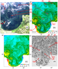
Finally, by 23 August the hydrometeorological conditions in the Southeastern Baltic Sea have drastically changed: a tight northeasterly wind promoted coastal upwelling and a related jet-like coastal current, which, in turn, shed cyclonic eddies behind/downstream topographic features such as the Sambian Rise (C14 and C15 cyclones in Figure 9), Cape Taran (C16 and C17), and Cape Rozewie (C18).
 |
| Table 1 |
The information about the evolution of the above-mentioned mesoscale eddies including the date and place of their birth/decay, life path, and life time is summarized in Table 1.
Satellite monitoring of the Southeastern Baltic Sea is seriously affected by cloudiness, which prevents receiving information on ocean dynamics. According to the authors' estimates based on the data obtained from the online Giovanni system developed and maintained by the Goddard Earth Sciences Data and Information Services Center at NASA (http://disc.sci.gsfc.nasa.gov/giovanni), this region is partially or completely covered by clouds approximately 60% of the year [Ginzburg et al., 2015a]. SAR imagery allows detecting some signatures of ocean dynamics in cloudy conditions, but there are certain restrictions caused by weather conditions and problems in the interpretation of SAR images [Lavrova et al., 2011, 2016]. In such circumstances, high resolution numerical models seem to be the best tool to reproduce daily mesoscale and sub-mesoscale fields of currents in the cloudy conditions typical for the Baltic Sea.
The above-presented comparison of the satellite imagery against the model output revealed reasonably good correspondence between the observed and simulated patterns of the mesoscale eddy fields in the surface layer of the Southeastern Baltic Sea for the period of May–August 2015. In our opinion, it has two consequences. First, the ultra-high resolution circulation model we implemented can be used for the hindcast and operational forecast of mesoscale eddy fields in the Southeastern Baltic Sea. Second, as the model has reproduced a handful of satellite images available for the period, one can expect that the simulation provides realistic information on the evolution of mesoscale and submesoscale eddies in the area, including the place and time of birth, size, intensity, track, life time, etc.
According to modeling results presented in Table 1, the tip of the Hel Spit is a special place for the Southeastern Baltic Sea where long-living mesoscale eddies and vortex pairs frequently originate. For example, the A1–C1 vortex pair was generated from a protuberance that protruded northward from the tip of the Hel Spit after a southeasterly wind gale. Then a newborn cyclone, C2, broke away from the tip of the Hel Spit, moved northward to meet and merge with C1, and thereby formed a modified vortex pair, A1–C2. In the course of time, the C2 cyclone detached from the A1 anticyclone and moved further north, while a newborn cyclone, C5, of the same place of origin (the tip of the Hel Spit) approached A1 to form the A1–C5 vortex pair. Note that the formation of a vortex pair north of the Hel Spit was first reported in [Zhurbas et al., 2004b] based on IR satellite images and model results.
The following question arises: What makes the tip of the Hel Spit a special place where mesoscale eddies are formed? Taking a look at a close-up of the Southeastern Baltic Sea bathymetry (Figure 1, right panel), one can admit that the tip of the Hel Spit is characterized by an exceptionally steep bottom slope, so that the 70 m depth contour (the level of the upper boundary of the permanent halocline) approaches the shore as close as 1–2 km. In such circumstances, relatively short-term exposure to the upwelling/downwelling favorable wind promotes a perturbation (bending) of the permanent halocline; as a result, mesoscale vortices are more powerful and long-living.
The eddies listed in Table 1 are mostly cyclones rather than anticyclones (16 cyclones vs 2 anticyclones). However, this does not mean that the number of cyclonic eddies in the surface sea layer exceeds that of anticyclonic eddies. In our opinion, the only thing that is beyond doubt is that the cyclonic eddies are better visualized on satellite and simulated images, having a larger angular velocity of rotation and a longer life time (e.g. [Väli et al., 2017]), and manifesting themselves in the form of easily noticeable spirals [Munk et al., 2000].
Finally, the results of simulation of submesoscale circulation in the Southeastern Baltic Sea are very promising for numerical modeling of oil pollution in this region. Since 2004, this area is under daily satellite monitoring of oil pollution related to oil production at the D-6 offshore oil platform operated by Lukoil-Kaliningradmorneft Ltd [Bulycheva et al., 2014, 2016; Kostianoy, 2006, 2015; Krek et al., 2018]. In the framework of this satellite monitoring, the Seatrack Web (STW) oil spill model of the Swedish Meteorological and Hydrological Institute (SMHI) is used for modeling the drift and transformation of observed oil spills since 2004. Today, STW is the official HELCOM forecast and hindcast system, which is used by national authorities and research organisations for calculating the fate of oil spills in the Baltic Sea since the 1990s. Our 15 year-long experience in using STW showed that the model does not provide a correct forecast for oil spill drift in this region in the presence of mesoscale and submesocale eddies, which are shown above to be characteristic of the Gulf of Gdansk [Ginzburg et al., 2015b]. Based on the above-reported results, the increase in the horizontal resolution in the SMHI operational circulation model coupled with STW is believed to be capable of significantly improving the quality of the forecast of oil spill drift in mesoscale and submesoscale eddy fields.
Bulycheva, E. V., A. V. Krek, A. G. Kostianoy, A. V. Semenov, A. Joksimovich (2016), Oil pollution in the Southeastern Baltic Sea by satellite remote sensing data in 2004–2015, Transport and Telecommunication, 17, no. 22, p. 155–163, https://doi.org/10.1515/ttj-2016-0015.
Bulycheva, E., I. Kuzmenko, V. Sivkov (2014), Annual sea surface oil pollution of the south-eastern part of the Baltic Sea by satellite data for 2006–2013, Baltica, Special Issue, 27, p. 9–14, https://doi.org/10.5200/baltica.2014.27.10.
Burchard, H., K. Bolding (2001), Comparative Analysis of Four Second-Moment Turbulence Closure Models for the Oceanic Mixed Layer, J. Phys. Oceanogr., 31, p. 1943–1968, https://doi.org/10.1175/1520-0485(2001)031%3C1943:CAOFSM%3E2.0.CO;2.
Burchard, H., K. Bolding (2002), GETM – a general estuarine transport model. Scientific documentation. Technical report EUR 20253en., European Commission, Ispra, Italy.
Canuto, V. M., et al. (2001), Ocean Turbulence. Part I: One-Point Closure Model-Momentum and Heat Vertical Diffusivities, J. Phys. Oceanogr., 31, p. 1413–1426, https://doi.org/10.1175/1520-0485(2001)031%3C1413:OTPIOP%3E2.0.CO;2.
Dabuleviciene, T., I. Kozlov, D. Vaiciute, I. Dailidiene (2018), Remote sensing of coastal upwelling in the South-Eastern Baltic Sea: Statistical properties and implications for the coastal environment, Remote Sensing, 10, no. 11, p. 1752, https://doi.org/10.3390/rs10111752.
Elkin, D. N., A. G. Zatsepin (2013), Laboratory Investigation of the Mechanism of the Periodic Eddy Formation Behind Capes in a Coastal Sea, Oceanology, 53, no. 1, p. 24–35, https://doi.org/10.1134/S0001437012050062.
Ginzburg, A. I., E. V. Bulycheva, A. G. Kostianoy, D. M. Solovyov (2015a), Vortex Dynamics in the Southeastern Baltic Sea from Satellite Radar Data, Oceanology, 55, no. 6, p. 805–813, https://doi.org/10.1134/S0001437015060065.
Ginzburg, A. I., E. V. Bulycheva, A. G. Kostianoy, D. M. Solovyov (2015b), On the role of vortices in the transport of oil pollution in the Southeastern Baltic Sea (according to satellite monitoring), Current Problems in Remote Sensing of the Earth From Space, 12, no. 3, p. 149–157 (in Russian).
Ginzburg, A. I., A. G. Kostianoy, D. M. Soloviev, S. V. Stanichny (1998), Upwelling cyclonic eddies off south-western tip of the Crimea, Issledovanie Zemli iz Kosmosa, 3, p. 83–88 (in Russian).
Ginzburg, A. I., E. V. Krek, A. G. Kostianoy, D. M. Solovyev (2017), Evolution of mesoscale anticyclonic vortex and vortex dipoles/multipoles on its base in the south-eastern Baltic (satellite information May–July 2015), Journal of Oceanological Research, 45, no. 1, p. 10–22, https://doi.org/10.29006/1564-2291.JOR-2017.45(1).3 (in Russian).
Gräwe, U., P. Holtermann, K. Klingbeil, H. Burchard (2015), Advantages of vertically adaptive coordinates in numerical models of stratified shelf seas, Ocean Modelling, 92, p. 56–68, https://doi.org/10.1016/j.ocemod.2015.05.008.
Gurova, E., A. Lehmann, A. Ivanov (2013), Upwelling dynamics in the Baltic Sea studied by a combined SAR/infrared satellite data and circulation model analysis, Oceanologia, 55, no. 3, p. 687–707, https://doi.org/10.5697/oc.55-3.687.
Hofmeister, R., H. Burchard, J.-M. Beckers (2010), Non-uniform adaptive vertical grids for 3D numerical ocean models, Ocean Modelling, 33, no. 1–2, p. 70–86, https://doi.org/10.1016/j.ocemod.2009.12.003.
Johansson, J. (2018), Total and regional runoff to the Baltic Sea, HELCOM Baltic Sea Environment Fact Sheets, Online data, HELCOM, Helsinki, Finland (http://www.helcom.fi/baltic-sea-trends/ environment-fact-sheets/).
Karimova, S. S., O. Yu. Lavrova, D. M. Solov'ev (2012), Observation of Eddy Structures in the Baltic Sea with the Use of Radiolocation and Radiometric Satellite Data, Izvestiya, Atmospheric and Oceanic Physics, 48, no. 9, p. 1006–1013, https://doi.org/10.1134/S0001433812090071.
Kostianoy, A. G. (2017), Satellite monitoring of the ocean climate parameters. Part 1, Fundamental and Applied Climatology, 2, p. 27–49, https://doi.org/10.21513/2410-8758-2017-2-63-85 (in Russian).
Kostianoy, A. G., et al. (2006), Operational satellite monitoring of oil spill pollution in the southeastern Baltic Sea: 18 months experience, Environmental Research, Engineering and Management, 4, no. 38, p. 70–77.
Kostianoy, A. G., E. V. Bulycheva, A. V. Semenov, A. V. Krainyukov (2015), Satellite monitoring systems for shipping, and offshore oil and gas industry in the Baltic Sea, Transport and Telecommunication, 16, no. 2, p. 117–126, https://doi.org/10.1515/ttj-2015-0011.
Krauss, W., B. Brügge (1991), Wind-produced water exchange between the deep basins of the Baltic Sea, J. Phys. Oceanogr., 21, p. 373–384, https://doi.org/10.1175/1520-0485(1991)021%3C0373:WPWEBT%3E2.0.CO;2.
Krek, E., A. Kostianoy, A. Krek, A. V. Semenov (2018), Spatial distribution of oil spills at the sea surface in the Southeastern Baltic Sea according to satellite SAR data, Transport and Telecommunication, 19, no. 4, p. 294–300, https://doi.org/10.2478/ttj-2018-0024.
Lavrova, O. Yu., E. V. Krayushkin, K. R. Nazirova, A. Ya. Strochkov (2018), Vortex structures in the Southeastern Baltic Sea: Satellite observations and concurrent measurements, Proc. SPIE 10784, Remote Sensing of the Ocean, Sea Ice, Coastal Waters, and Large Water Regions 2018, 1078404 (5 October 2018), https://doi.org/10.1117/12.2325463.
Lavrova, O. Yu., A. G. Kostianoy, S. A. Lebedev, M. I. Mityagina, A. I. Ginzburg, N. A. Sheremet (2011), Complex Satellite Monitoring of the Russian Seas, 470 pp., IKI RAN, Moscow (in Russian).
Lavrova, O. Yu., M. I. Mityagina, A. G. Kostianoy (2016), Satellite Methods of Detection and Monitoring of Marine Zones of Ecological Risks, 336 pp., Space Research Institute, Moscow (in Russian).
Lehmann, A., K. Myrberg (2008), Upwelling in the Baltic Sea – A review, J. Mar. Syst., 74, p. S3–S12, https://doi.org/10.1016/j.jmarsys.2008.02.010.
Lips, U., V. Zhurbas, M. Skudra, G. Väli (2016), A numerical study of circulation in the Gulf of Riga, Baltic Sea. Part I: Whole-basin gyres and mean currents, Cont. Shelf Res., 112, p. 1–13, https://doi.org/10.1016/j.csr.2015.11.008.
Männik, A., M. Merilain (2007), Verification of different precipitation forecasts during extended winter-season in Estonia, HIRLAM Newsletter , 52, p. 65–70.
Munk, W. H., L. Armi, K. Fischer, F. Zachariasen (2000), Spirals on the sea, Proc. R. Soc. Lond., A 456, p. 1217–1280.
Myrberg, K., O. Andrejev (2003), Main upwelling regions in the Baltic Sea – A statistical analysis based on three-dimensional modeling, Boreal Environment Research, 8, no. 2, p. 97–112.
Umlauf, L., H. Burchard (2005), Second-order turbulence closure models for geophysical boundary layers. A review of recent work, Cont. Shelf Res., 25, no. 7–8, p. 795–827, https://doi.org/10.1016/j.csr.2004.08.004.
Väli, G., V. Zhurbas, U. Lips, J. Laanemets (2017), Submesoscale structures related to upwelling events in the Gulf of Finland, Baltic Sea (numerical experiments), J. Mar. Syst., 171, no. SI, p. 31–42, https://doi.org/10.1016/j.jmarsys.2016.06.010.
Väli, G., V. M. Zhurbas, J. Laanemets, U. Lips (2018), Clustering of floating particles due to submesoscale dynanics: a simulation study for the Gulf of Finland, Fundamentalnaya i Prikladnaya Gidrofizika, 11, no. 2, p. 21–35, https://doi.org/10.7868/S2073667318020028.
Vignudelli, S., A. Kostianoy, P. Cipollini, J. Benveniste (eds.) (2011), Coastal Altimetry, 578 pp., Springer-Verlag, Berlin, Heidelberg, https://doi.org/10.1007/978-3-642-12796-0.
Zhurbas, V., J. Elken, V. Paka, J. Piechura, I. Chubarenko, N. Golenko, S. Shchuka (2012), Structure of unsteady overflow in the Slupsk Furrow of the Baltic Sea, J. Geophys. Res. – Oceans, 117, no. C04027, p. 1–17, https://doi.org/10.1029/2011JC007284.
Zhurbas, V. M., N. P. Kuzmina, D. A. Lyzhkov (2017), Eddy formation behind a coastal cape in a flow generated by transient longshore wind (numerical experiments), Oceanology, 57, no. 3, p. 350–359, https://doi.org/10.1134/S0001437017020229.
Zhurbas, V., I. S. Oh, T. Park (2006), Formation and decay of a longshore baroclinic jet associated with transient coastal upwelling and downwelling: A numerical study with applications to the Baltic Sea, J. Geophys. Res., 111, no. C04014, p. 1–18, https://doi.org/10.1029/2005JC003079.
Zhurbas, V., T. Stipa, P. Mälkki, I. Hense, V. Sklyarov, et al. (2004a), Generation of subsurface cyclonic eddies in the southeast Baltic Sea: Observations and numerical experiments, J. Geophys. Res., 109, no. C05033, p. 1–12, https://doi.org/10.1029/2003JC002074.
Zhurbas, V. M., T. Stipa, P. Mälkki, V. T. Paka, N. P. Kuzmina, V. E. Sklyarov (2004b), Mesoscale Variability of Upwelling in the South-East Baltic: Infrared Images and Numerical Modeling, Oceanology, 44, no. 5, p. 619–628.
Zhurbas, V., G. Väli, M. Golenko, V. Paka (2018), Variability of bottom friction velocity along the inflow water pathway in the Baltic Sea, J. Mar. Syst., 184, p. 50–58, https://doi.org/10.1016/j.jmarsys.2018.04.008.
Received 18 April 2019; accepted 13 June 2019; published 22 August 2019.

Citation: Zhurbas Victor, Germo Väli, Andrey Kostianoy, Olga Lavrova (2019), Hindcast of the mesoscale eddy field in the Southeastern Baltic Sea: Model output vs satellite imagery, Russ. J. Earth Sci., 19, ES4006, doi:10.2205/2019ES000672.
Copyright 2019 by the Geophysical Center RAS.