RUSSIAN JOURNAL OF EARTH SCIENCES, VOL. 19, ES2004, doi:10.2205/2019ES000655, 2019
E. G. Morozov1, D. I. Frey1, N. A. Diansky2,3,4, V. V. Fomin3
1Shirshov Institute of Oceanology RAS, Moscow, Russia
2Lomonosov Moscow State University, Moscow, Russia
3Zubov State Oceanographic Institute, Moscow, Russia
4Institute of Numerical Mathematics RAS, Moscow, Russia
We study bottom circulation in the Norwegian Sea in the region of nuclear submarine wreck. A numerical model (INMOM) with a high vertical and horizontal resolution in the bottom layers is applied for the estimates of bottom velocities and direction of currents as well as their stability. The model revealed that the currents in the bottom layer of the Norwegian Sea are not strong. The fluctuations of currents with periods of 5–6 days and 12 hours are several times greater than the mean currents in the region, which are of the order of 1 cm/s excluding the region of the Bear Island Trough.
Circulation in the Norwegian Sea has been studied in many publications. They are mostly related to the surface currents and intermediate depths. A review can be found in [Filyushkin et al., 2018]. This research deals with the bottom circulation in the Norwegian Sea related to the catastrophic sinking of nuclear submarine "Komsomolets" 30 years ago. There are several publications related to this catastrophe and spreading of currents in the region [Aleinik et al., 1999, 2002; Fomin et al., 1996; Lukashin and Shcherbinin, 2007; Sidorova and Shcherbinin, 2004].
Nuclear submarine "Komsomolets" sank in the Norwegian Sea on 7 April 1989 at a point about 180 nautical miles southwest of Bear Island at a depth of about 1690 m approximately at 73° 44$'$ N, 13° 16$'$ E [Vinogradov et al., 1996]. It is a potential hazard to the environment due to the possible radioactive contamination from the reactor and the nuclear torpedo warheads. There were plans to salvage the submarine totally, to salvage the torpedo part, or to seal off the torpedo part of the submarine. However, the current decision to protect the nature from contamination is to leave "Komsomolets" where it is [Blindheim et al., 1994].
Dangerous radioactive components, which may be dissolved in seawater and spread in the sea, include cesium-137 and strontium-90. Plutonium, which is almost not dissolved in water will settle in the sediments and remain there for long. This research is an attempt to analyze how radioactive elements would spread if a leakage occurs. The study is based on numerical modeling and moored measurements of currents. Previous studies resulted in conclusions that the nuclear submarine is a minor radioactive pollution problem because the amount of radioactive material is relatively small, the wreck sank at a very deep location, and the amount of water for dilution is the whole sea [Blindheim et al., 1994]. The possible radioactivity will spread in the water at great depths at isopycnic surfaces. Previous researches revealed that the currents in the region are not uniform but fluctuating [Fomin et al., 1996]. Possible radioactive pollution will remain in the deep water and will be diluted slowly. It is not possible that polluted deep water will ascent to the surface from a depth of about 1700 m. The concentration of pollution in the water will not be high even if a leakage occurs. The residence time of the circulation system is estimated as a few centuries [Blindheim et al., 1994].
In this study we apply a numerical model to estimate the velocities of bottom currents in the region of catastrophe and compare the simulation results with the direct measurements of currents on moorings and previous results.
We applied the Institute of Numerical Mathematics Ocean Model (INMOM) to simulate the circulation in the bottom layer of the Norwegian Sea [Diansky et al., 2002; Marchuk et al., 2005; Zalesny et al., 2012]. This model is based on the system of the so-called primitive ocean hydrodynamics equations in spherical horizontal coordinates. We apply the hydrostatic and Boussinesq approximations and the vertical $\sigma$-coordinate system. The horizontal components of the velocity vector, potential temperature, salinity, and fluctuations of the sea surface height above the mean sea level are the prognostic variables of the model. Seawater density is calculated from the equation of state with the account for water compression [Brydon et al., 1999]. The realization of the model is based on the splitting method with respect to the physical processes and, when possible, with respect to the spatial coordinates [Marchuk et al., 2005]. Application of this method makes the model different from other well-known ocean models. The thermo-hydrodynamic equations of the model are written in a special symmetrized form so that it is possible to split the operator of the full problem into a set of simpler operators and construct spatial approximations of the relevant groups of summands (in different equations). All the split discrete problems satisfy the energy conservation law, which is valid for the initial differential problem. The simulation domain is between 00° 00$'$ E and 40° 00$'$ E and between 69° 00$'$ N and 80° 00$'$ N, or 400 by 220 computational grid nodes. The vertical resolution was determined by the need to simulate the circulation in the bottom layer. The vertical coordinate of the INMOM sigma-model is determined by relation
\begin{eqnarray*} \sigma = \frac{z-\zeta}{H-\zeta} \end{eqnarray*}where $z$ is the traditional downward vertical coordinate, $H$ is the ocean depth at the given point, and $\zeta$ is sea surface height relative to its unperturbed state. The application of sigma-levels is especially efficient for the simulation of the bottom circulation and rough bottom topography because it makes modeling bottom oceanic domains possible at significantly variable depths within one simulation [Diansky et al., 2002].
In our simulation, we selected 36 vertical levels; the model resolution increased with depth for better simulation of the bottom currents. The lower 15 sigma-levels were specified in the bottom layer. The distance between them was about 40 m at the depth of the location of the wreck; the vertical resolution depends on the ocean depth, which varied between the coastal regions and 4000 m. The ability of the INMOM model to reproduce circulation with a high spatial resolution under the condition of steep bottom topography is shown in [Diansky et al., 2013].
The bottom topography was taken from the GEBCO2013 database (https://www.gebco.net/ data_and_products/gridded_bathymetry_data/). The horizontal resolution of the grid is 30 arc-second. The initial conditions for the temperature and salinity field were specified from the climatic monthly mean data of atlas [Locarnini et al., 2010]. The initial velocity fields and sea surface height deviations were set zero (state of rest). These data were also used to specify the annual cycle of temperature and salinity at liquid boundaries. The heat and salt fluxes at the surface are supplemented by the relaxation additives to fit the model temperature and salinity values to the climatic data using the "nagging" method with a coefficient of $\sim 50$ m/yr [Diansky et al., 2002].
The results of simulations were compared with the available field observations at several moorings in the region. The measurements were also compared with the data of the CTD/LADCP profilers, which measure profiles of the thermohaline characteristics and current velocities, respectively. Processing of the temperature and salinity data was performed using the standard SBE Data Processing programming code package (Sea-Bird Electronics, SBE 19plus SeaCAT Profiles CTD User Manual, Release Date 08/27/2016. http://www.seabird.com/).
The results of model simulations are shown in Figure 1, which presents the vectors of currents in the bottom layer. The bottom currents were simulated for two seasons in January and July. Both charts show that bottom currents are quite low and generally there are no jets of high velocity in the entire sea except for the bottom stream of the bottom water from the Barents Sea flowing from the Bear Island Trough. This stream turns to the north around Spitsbergen. These conclusions are consistent with the conclusions made on the basis of direct measurements in the Bear Island Trough in 2017 [Frey et al., 2017]. A chart of velocity vectors in [Filyushkin et al., 2018] shows vectors of currents at a depth of 1500 m based on the ARGO data. It is worth noting that at this depth individual jets can flow into the Bear Island Trough. Hence, there is a possibility of the existence of compensating bottom currents down the canyon. We also note that cold and dense waters are not formed in the Barents Sea, but they can be formed on the slopes of Spitsbergen.
In this paper we analyze the results of velocity measurements on moorings deployed in the vicinity of the wreck:
|
| Figure 2 |
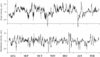
Time series of the zonal and meridional components of the currents near the bottom measured on mooring 2 are shown in Figure 2.
Velocity components fluctuate with a period of a few days. The speed generally does not exceed 15 cm/s. The mean velocities over the entire period of measurements on both moorings are within 1 cm/s directed to the northeast. This is confirmed by the progressive vector diagram shown in Figure 3 based on the measurements in August, 1995 at point 1. Water particles displace over a distance not exceeding 100 km during one month. This conclusion coincides with the conclusions made by [Aleinik et al., 1999].
 |
| Figure 4 |
Higher frequency fluctuations of velocity can be seen from the analysis of power spectra of these fluctuations. Graphs of power spectra of the zonal and velocity components of currents measured close to the bottom on mooring are shown in Figure 4. A prominent semidiurnal tidal peak is clearly seen on both graphs. The periods of inertial and semidiurnal $M_2$ periods at this latitude do not make possible their separation. In addition fluctuations with a period of 5–6 days give a contribution to the fluctuations of the mesoscale range, which can be caused by the internal dynamics of the ocean in this region.
Modeling simulation using the INMOM model with a high vertical and horizontal resolution in the bottom layers revealed that the currents in the bottom layer of the Norwegian Sea are not strong excluding the region of the continental slope of Spitsbergen where a jet of the Arctic waters flowing from the Bear Island Trough turns to the north. The fluctuations of currents with periods of 5–6 days and 12 hours are several times greater than the mean currents in the region which are of the order of 1 cm/s. The results of the model simulation with a high resolution model tuned to simulate the bottom currents confirm the results of previous research that the nuclear submarine on the bottom of the Norwegian Sea is a minor radioactive pollution problem because there is no leakage of the radioactive substance. If unfortunately such a leakage starts the deep location of the wreck will not produce much harm because the amount of water for dilution is enormous. The possible radioactive pollution will remain in the deep water and will be diluted slowly. It is not possible that polluted deep water would ascent to the surface from a depth of about 1700 m. The currents in the region are not uniform but fluctuating; hence polluted water will only slowly spread from this region.
Aleinik, D. L., V. I. Byshev, A. D. Shcherbinin (1999), Measured currents in the near-bottom layer of the Norwegian Sea within the region of catastrophe of the atomic submarine Komsomolets, Doklady Earth Sciences, 369, no. 9, p. 1393–1397.
Aleinik, D. L., V. I. Byshev, A. D. Shcherbinin (2002), Water Dynamics in the Norwegian Sea at the site of the accident of the Komsomolets nuclear submarine, Oceanology, 42, no. 1, p. 7–16.
Blindheim, J., L. Føyn, E.A. Martinsen, E. Svendsen, R. Sætre (1994), The sunken nuclear submarine in the Norwegian Sea – A potential environmental problem? Research report, Institute of Marine Research, Bergen (https://brage.bibsys.no/xmlui/handle/11 250/112899).
Brydon, D., S. San, R. Bleckb (1999), A new approximation of the equation of state for seawater, suitable for numerical ocean models, J. Geophys. Res., 104, no. C1, p. 1537–1540, https://doi.org/10.1029/1998JC900059.
Diansky, N. A., A. V. Bagno, V. B. Zalesny (2002), Sigma model of global ocean circulation and its sensitivity to variations in wind stress, Izv., Atmos. Ocean. Phys., 38, no. 4, p. 537–556.
Diansky, N. A., V. V. Fomin, N. V. Zhokhova, A. N. Korshenko (2013), Simulations of currents and pollution transport in the coastal waters of Big Sochi, Izv., Atmos. Ocean. Phys., 49, no. 6, p. 611–621, https://doi.org/10.1134/S0001433813060042.
Filyushkin, B. N., M. A. Sokolovskiy, K. V. Lebedev (2018), Evolution of an intrathermocline lens over the Lofoten Basin, The Ocean in Motion, M. G. Velarde, R. Yu. Tarakanov, A. V. Marchenko (eds.), p. 333–347, Springer Oceanography, https://doi.org/10.1007/978-3-319-71934-4_21.
Fomin, L. M., A. D. Shcherbinin, K. G. Vinogradova, K. V. Lebedev, et al. (1996), Currents in the Northeastern Part of the Norwegian Sea from the Results of Direct Measurements, Oceanological Studies and Underwater and Engineering Operations at the Site of the Accident of the Komsomolets Nuclear Submarine, M. E. Vinogradov, A. M. Sagalevich, and S. V. Khetagurov (eds.), p. 263–287, Nauka, Moscow (in Russian).
Frey, D. I., A. N. Novigatsky, M. D. Kravchishina, E. G. Morozov (2017), Water structure and currents in the Bear Island Trough in July–August 2017, Russ. J. Earth. Sci., 17, p. ES3003, https://doi.org/10.2205/2017ES000602.
Locarnini, R. A., A. V. Mishonov, J. I. Antonov, et al. (2010), World Ocean Atlas 2009, Vol. 1: Temperature, U.S. Government Printing Office, Washington, D.C.
Lukashin, V. N., A. D. Shcherbinin (2007), Hydrological properties, suspended matter, and particulate fluxes in the water column of the Bear Island Trough, Oceanology, 47, no. 1, p. 68–79, https://doi.org/10.1134/S0001437007010109.
Marchuk, G. I., A. S. Rusakov, V. B. Zalesny, N. A. Diansky (2005), Splitting numerical technique with application to the high resolution simulation of the Indian ocean circulation, Pure Appl. Geophys., 162, p. 1407–1429, https://doi.org/10.1007/s00024-005-2677-8.
Sidorova, A. N., A. D. Shcherbinin (2004), Intra-annual variability of the thermohaline structure and circulation in the Barents Sea based on the results of model calculations, Oceanology, 44, no. 5, p. 629–637.
Vinogradov, M. E., et al. (eds.) (1996), Oceanological Studies and Underwater and Engineering Operations at the Site of the Accident of the Komsomolets Nuclear Submarine, Nauka, Moscow.
Zalesny, V. B., N. A. Diansky, V. V. Fomin, S. N. Moshonkin, S. G. Demyshev (2012), Numerical model of the circulation of the Black Sea and the Sea of Azov, Russian Journal of Numerical Analysis and Mathematical Modelling, 27, no. 1, p. 95–111, https://doi.org/10.1515/rnam-2012-0006.
Received 6 December 2018; accepted 18 December 2018; published 19 March 2019.

Citation: Morozov E. G., D. I. Frey, N. A. Diansky, V. V. Fomin (2019), Bottom circulation in the Norwegian Sea, Russ. J. Earth Sci., 19, ES2004, doi:10.2205/2019ES000655.
Copyright 2019 by the Geophysical Center RAS.