
RUSSIAN JOURNAL OF EARTH SCIENCES, VOL. 19, ES1001, doi:10.2205/2018ES000642, 2019
Evgeny Krayushkin, Olga Lavrova, Alexey Strochkov
Space Research Institute of Russian Academy of Sciences, Moscow, Russia
This paper describes our experience in the application of Lagrangian mini-drifters in studies of coastal water circulation. As shown by our experiments in the Southeastern Baltic Sea, an application of Lagrangian mini-drifters makes it possible to detect the presence of complex sub-mesoscale vortex processes and inertial oscillations, i.e., processes that are difficult to numerically simulate. Moreover, the presence of vortex formations is able to keep passive objects (drifts, oil anthropogenic pollution and so on) floating in a strictly localized area for at least 1 week, even in changeable wind conditions. Special attention in the paper is paid to a performance comparison of the application of mini-drifters and an Acoustic Doppler Current Profiler (ADCP). The advantages of drifters for determining flow parameters at low speeds are noted. The main advantages of the proposed drifters are taken into account: the low cost of manufacturing drifters ($\sim 150$ USD per system) along with the low cost of GSM communications, the ease of manufacturing and operation, with no special technical experience required, and the link to obtaining operational data in real-time for up to several weeks make these systems valuable supplementary tools for remote sensing studies of processes in coastal zones.
The ecological situation of coastal zones is one of the major concerns in modern science. This is due to many factors: the increase of oil pollution caused by an increase in oil and gas activity on the shelf, intensification of commercial shipping and an increase of suspended matter concentration, which drives a decrease of bioproductivity and an increase of harmful algae blooming. One of the most important questions for ecological monitoring is not only the detection of anthropogenic and natural pollutants but also the forecasting of their propagation in time. A correct forecast is only possible if it is based on an understanding of the whole spectrum of hydrodynamic processes in the area. Bearing in mind the complexity and high costs of field experiments, we may assume that the variety of real-ocean situations and impact of a great amount of atmospheric and oceanic factors yield some fragmentarity in the description of real processes in the areas of interest [Lynch et al., 2015; Marmorino et al., 2010]. In order to forecast the propagation of different types of pollutions, it is necessary to obtain comprehensive detailed data of a near real-time spaciotemporal distribution of different meso and submesoscale processes (eddies, vortex dipoles, internal waves, fronts, etc.) [Ginzburg et al., 2015a, 2015b; Lavrova et al., 2016]. The submesoscale phenomena are too complex to be studied due to their non-stationarity, spontaneity of their appearance and their relatively short lifetime.
There are many methods for studying coastal dynamics and submesoscale processes, including in-situ methods, numerical modelling and remote sensing data. In modern science, numerical modelling is considered to be the most popular and comprehensive tool for studying dynamic processes in coastal zones. As examples, we can mention the Princeton Ocean Model, and its modifications for various seas [Blumberg et al., 1987; Jankowski et al., 2002; Svendsen et al., 1996; Zhurbas et al., 2003, 2004], the NEMO-Nordic model (Nucleus of the European Modeling of the Ocean) [Madec et al., 1998], which was set up for the North Sea and the Baltic Sea [Hordoir et al., 2013; Madec, 2008], and many others. The main advantages of numerical simulation are the data coverage of wide areas (averaged according to different time scales) and the possibility to predict current fields in time. However, for coastal water circulation, the results of numerical simulation require a more detailed analysis, with additional involvement of verification based on in-situ data.
Oceanographic in-situ methods for studying currents can be divided into two parts. The first technique is based on Euler's approach, when the flow passes over a fixed point. The main types of instruments used in this approach are impeller current meters, which determine the speed of the current through the frequency of the impeller shaft movement in time, and an Acoustic Doppler Current Profiler (ADCP), which determines the flow velocity through the Doppler shift by means of acoustic signals. Both devices are widely used in oceanographic researches [Joseph, 2014], but can measure only at a fixed point. However, coastal dynamics is characterized by a high degree of spatiotemporal variability and cannot be fully described using several fixed-point measurements. Additionally, most bottom-mounted ADCP devices do not measure the upper meters of water columns due to an acoustic blind zone near the surface. The second method for describing currents is the Lagrangian approach, when an object follows a certain water parcel. Sequential mapping of the object's location in space at regular intervals helps to create the flow lines of a dynamic field. The main types of instruments for researching the flow field by the Lagrangian method is a Lagrangian drifter and shore-based HF radars [Carlson et al., 2010; LaCase, 2008]. HF radars are very comprehensive measuring devices, which provide real-time currents and wave data over a vast coastal zone area, but they are quite expensive and difficult to install. We will emphasize the Lagrangian drifter – passive floating object, with or without an underwater sail and a minimized windage area. Drifters can be equipped with a remote data-transmitting device (satellite, radio or cellular link) to transmit data in real time or can store data internally. An advantage of the application of Lagrangian drifters is the possibility to cover vast areas with drifting buoys, and the cost of a single instrument is relatively low. The ability to send data in real-time and follow currents at different depths (if using underwater sails at different depths) makes these instruments very attractive for research processes in coastal areas.
The most complete description of drifter experiments can be found in [Lumpkin et al., 2017]. A sufficient improvement of the application of Lagrangian drifters for the task of studying the field of currents is associated with the advent of the ubiquitous GPS satellite tracking system in the 1970s. A pioneering research in the application of Lagrangian drifters for studying flow fields was conducted by Niiler and co-authors [Niiler et al., 1987]. They launched underwater sail drifters, equipped with Argos satellite receivers off the coast of California. Sybrandy and Niiler [Sybrandy and Niilier, 1991] also presented a guide to developing Lagrangian drifters and recommendations for the optimization of drifter experiments. Poulain and co-authors [Poulain et al., 2005] conducted extensive research by launching 54 Lagrangian drifters, equipped with GPS and satellite communication receivers, in the Black Sea from 1999–2003. Results of this detailed research allowed for the description of the large-scale circulation of the Black Sea and revealed some distinctive features of the Black Sea surface circulation. Poje and co-authors described the submesoscale dispersion in the vicinity of the Deepwater Horizon spill after the Grand Lagrangian Deployment was launched, with 300 GPS-drifters in the Gulf of Mexico calculating the dispersion of the propagation of drifters in the DeSoto Canyon region [Poje et al., 2014]. Recent work [D'Asaro et al., 2018] showed the experience of calculating ocean convergence and the dispersion of flotsam for 200 drifters.
Despite the fact that an application of Lagrangian drifters using satellite telemetry provides a large array of useful information for investigating large-scale circulation, this technology is quite expensive and restricted in some countries or certain areas. The recently acquired possibility of transmitting information obtained by drifters via mobile phones (GSM) makes drifter experiments affordable for scientific groups with a constrained budget, who are engaged in studies of mesoscale and small-scale circulation in coastal zone areas covered by a cellular connection.
In this paper, we share our experience of designing low-budget Lagrangian drifters to study the dynamics of coastal water. We also show the applicability of such drifters for the determination of parameters of coastal circulation in comparison with other methods of investigating the flow field.
When using a Lagrangian drifter, the possibility to obtain data in real time is very important. First, in drifter experiments, there is a high possibility of losing a device during bad weather conditions or malicious acts, and, second, it is very important to get data in real time in order to understand a current hydrodynamic situation in the region. This defines the necessity of transmitting the information, obtained by a drifter, immediately after it has been received. Drifters with a cellular communication
(Global System for Mobile Communications, GSM) channel for data transmission are significantly cheaper than the satellite one, both with respect to the cost of the equipment as well as to the cost of data transfer. Given their low cost and the limited range of their GSM-link (usually 25 km away from the shore), we will henceforth refer to them as mini-drifters.
To study the dynamics of coastal waters, a mini-drifter should meet certain requirements. The direct effect of the near-surface wind, which often does not coincide with the direction of a current, should be minimized. This can be achieved by the implementation of an underwater sail in a certain area to transmit the impulse of the water flow to a drifting object. With a sufficient area of an underwater sail, the pulse of a flowing water volume overcomes the effect of the wind pulse, acting on the minimally projecting area above the water surface if the wind speed does not exceed 10 m/s [Davis, 1985]. This allows us to neglect the impact of near-surface winds. Finally, a drifter should be able to track the movement of water masses, not only in the surface layer itself, but also at a certain depth. To achieve this, it is necessary to apply a series of mini-drifters with an underwater sail at different investigated horizons and depths.
The following is a description of the mini-drifters that we have developed and used in our studies of the coastal currents in the Black and Baltic Seas.
|
| Figure 1 |
A schematic diagram of our mini-drifter is shown in Figure 1. The main working tool of a
mini-drifter is the GPS / GSM-tracker (marked with 1 in Figure 1) that determines the coordinates of a drifting object and transmits them to a receiving device via the mobile network as short text messages (SMS) or via the General Packet Radio Service (GPRS) channel to a remote server.
A box with the tracker is attached to a float (2 in Figure 1), from which a rope (3 in Figure 1), with a sail (4) and an attached load (5), is lowered to a required depth to determine the movement of water. An underwater sail, has frame, (6 in Figure 1), and two perpendicular blades.
As a transceiver in the mini-drifters, we use car trackers. This programmable device determines the coordinates of its location using the GPS receiver and transmits these coordinates over a mobile cellular communication system to a device, such as a mobile phone, a smartphone, a tablet or a computer.
The programming of a tracker is carried out by a sequence of SMS-messages, with commands that specify the settings of the tracker mode, or through commands via a remote web-interface.
Data can be hosted in real-time on a data server for quick view and can be further downloaded.
In our experiments, Lagrangian drifters have worked, on average, for at least two weeks without needing a battery replacement.
 |
| Figure 2 |
The launch of mini-drifters, as a rule, is carried out from a small research vessel (Figure 2). A limitation of the immediate transmission of data obtained by mini-drifters by cellular communication is, first of all, that a marine area is covered by a GSM signal. In the Russian waters of the southeastern part of the Baltic Sea, the GSM signal is available at 30 km from the coast.
Information gathered outside of a cellular range is stored on a memory card and can be transmitted when a mini-drifter returns to a zone with an available signal. As a result, mini-drifters can provide quite complete and objective information about the parameters of coastal currents at various horizons.
 |
| Figure 3 |
In July 2014, our field work on the Black Sea shelf, in the vicinity of the Gelendzhik City (Figure 3), included experimental launches of a series of mini-drifters, synchronized with the towing of the acoustic Doppler profiler ADCP by a small research vessel.
Four mini-drifters, with underwater sails of 1 m$\times 1$ m, were launched at a distance of about 150 m from each other. The sails were located, relative to the water surface, at depths of between 0.5 and 1.5 m, 4.2 and 5.2 m, 6.6 m and 7.6 m, and 15 and 16 m. The drifters with sails, located at a depth of between 15 and 16 m, were deployed, first, at a distance of about 1.5 km from the shore. Then, while moving to the seaside, the other drifters were alternately launched, with their sails located at decreasing depths of 6.6 and 7.6 m; 4.2 and 5.2 m; and 0.5 and 1.5 m. Drifters transmitted the coordinates of their location every 10 minutes via the GSM-channel as SMS-messages. Simultaneously, the vertical distribution of currents at a depth of 150 m was measured by the ADCP TRDI WorkHorse Sentinel 300 kHz from a small vessel. The first depth cell, measured by ADCP, was placed at a depth of 4 m, and the vertical spacing between cells was from 2 m up to 150 m. The ADCP measured current ensembles at a rate of 2 seconds, revealing the research vessel speed, which was approximately 1.2 m/s, and resulting in an overall spatial resolution of approximately 3 m. All currents within the vertical resolution cell were averaged over an interval of 80 ensembles. With this setup, the averaged standard deviation was 0.78 cm/s, with a spatial resolution of $\sim 200$ m in the direction of the movement of the small vessel. The weight of each measurement was taken to be the same within the averaging window due to the quasi-state motion of the vessel at the experiment sites. An autonomous GPS receiver, connected to a computer, was used to identify the coordinates of the vessel, and the internal ADCP compass was used as a heading source.
 |
| Figure 4 |
 |
| Figure 5 |
The routes of drifters in the experiment, on 3 July 2014, and the current field parameters, found by means of ADCP, are shown in Figure 4. The weather during the experiment was calm, resolving in southeastern winds with an average of 2 m/s magnitude, and the height of waves was not more than 1 m. The drifters moved mainly in the southeastern direction, but with different speeds because their sails were at different depths, which reflected different depth velocities. The drifter with a sail at depths of between 0.5 and 1.5 m (drifting time 7.5 hours) moved with an average speed of 0.45 m/s, showing the presence of a strong current in the coastal zone. With depth, the current velocity decreased, while the same direction was maintained. The drifter with a sail at depths of between 4.2 and 5.2 m (with a drifting duration of 3 hours) coincided with the upper cell of ADCP, showing an average drift velocity of 0.37 m/s. The drift speed almost completely matched the results of measurements using ADCP with the assumptions of the measurement precision (an error is 0.05 m/s). The drifter with a sail at a depth of between 6.6 and 7.6 m (with a drifting duration of 9 hours) moved at about the same speed as the drifter, whose sail was located higher. This indicates the presence of a quasi-homogeneous flow in the layer from the surface to a depth of 8 m, which was confirmed by vertical velocity profiles according to ADCP (Figure 5). The drifter with a sail recessed at 15 m (with a duration of drift of 27 hours) moved much slower than the others. Its average drift velocity was only 0.07 m/s.
A distribution of velocities and directions of currents on 3 July according to the ADCP survey, is shown in Figure 5. The starting points of drifters are marked with circles, whose color is the same as those shown in Figure 4. The current, according to ADCP measurements, was pressed to the shore, slightly weakening in the seaward part of the profile. The current velocity decreased uniformly to a depth of 20 m, where the minimum velocity was 0.1 m/s. At depths of the isotach of 0.1 m/s, the drifter was moving with a sail buried 15 m deep. As can be seen in Figure 4 and Figure 5, the differences in the absolute speeds of the drifter and ADCP data are not more than 0.03 m/s. However, the difference between the directions of motion of the drifter at a depth of 15–16 m and the direction obtained from the ADCP data is 30°–45°. We can explain such a difference by the fact that the ADCP poorly determines the direction of the current vector with a small current velocity due to the imperfection of the metrological properties of the magnetic compass of the instrument and the initial error of the method, caused by towing the ADCP with much higher boat velocities ($\geq 1$ m/s) than the measured current velocity.
A comparison of different methods of measuring the current characteristics shows a good agreement between the determination of the current vector, using Lagrangian mini-drifters, and the Euler approach, using ADCP, when the flow velocity is more than 5 cm/s. The comparison also shows a significant advantage of Lagrangian mini-drifters over ADCP technics, when the current speed is below 5 cm/s. The direction of the flow is determined much more accurately with the help of Lagrangian drifters, and the data of the towed ADCP are not reliable for studying currents with low velocities. Lagrangian mini-drifters are also capable of measuring the flow parameters closer to the water surface because ADCP has a blind zone, the magnitude of which is determined by the frequency of the acoustic signal.
 |
| Figure 6 |
Since 2014, we have carried out field experiments in the Russian waters of the southeastern part of the Baltic Sea (Figure 6). The main purpose of our field work is to determine the parameters of the dynamics of coastal waters. In August 2017, a number of experiments were conducted with mini-drifters to reveal the direct influence of the wind on the drift of the buoys. We launched eight mini-drifters, constructed according to the design, described above. The location of each drifter in real time was transmitted every 15 minutes via GSM communication as SMS messages. To determine the direct influence of the wind, a forecast of the drift of the buoys was determined using the interactive model, Seatrack Web HELCOM (https://stw.smhi.se/).
Initially, the Seatrack Web model was developed only to predict the drift and transformation of spills of various types of oil products in the Baltic Sea. Since 2014, the floating object has been added to the model to track lost buoys and other objects on the surface. When determining the propagation path of such objects, the so-called wind factor is taken into account. This is presented as a percentage of the floating object's drift due to a wind. Model simulations can be run forward as well as backwards in time. The system uses the forecasted wind and current fields to predict five days of the drift of oil or other particles in three dimensions, with a spatial resolution of one nautical mile and a time resolution of 15 min. It takes into account a wind field forecast (and a number of other meteorological parameters), updated every three hours, and currents. The force fields of Seatrack Web HELCOM are presently provided by the weather model, HIRLAM, and the ocean model, HIROMB [Ambjörn et al., 2011; Liungman, O., Mattsson, J., Scientific documentation of Seatrack Web; physical processes, algorithms and references, 2011. Available online: http://www.smhi.se/polopoly$_$fs/1.15600!STW$_$ scientific$_$documentation.pdf (accessed on 11 July 2018)].
HELCOM Seatrack Web is fully operational and available 24/7 to everyone with a login access. The modeling results were provided to us in the framework of the environmental monitoring by LUKOIL-KMN Ltd.
 |
| Figure 7 |
Let us take a look at the results of our experiment, conducted on 27 August 2017. The buoy with an underwater sail of 1 m$^2$, located at a depth of 5 m (from 4.5 to 5.5 m) under the surface of the water, was launched at 14:00 GMT. The buoy was sending information until 03:39 GMT on 29 August 2017. The trajectory of the drift of the buoy during this period is shown in Figure 7. The average drift rate was 12 cm/s.
Since the temporal steps of the calculated fields by the Seatrack Web model is 15 minutes, the starting time of the buoy (27.08.2017, at 14:00 UTC) was taken as the start of the model forecast, and the end was considered to be 03:45 UTC on 29 August 2013, i.e., closest to the time of 03:39, at which point the drifting ended. Three model calculations were performed, with different wind factor values: 0% (no wind effect), 5% and 10%. This is a parameter that determines the direct effect of wind on a floating object, taking into account its surface sail. The trajectories of the model forecast of the buoy drift, with different wind factor values, are shown in Figure 7 by differently colored points.
The model forecast showed that the closest calculated drift trajectory of the floating object to the in-situ data was with a zero wind factor (see Figure 7). With wind factors of 5 and 10%, the drift velocity of the model object is 47 cm/s and 75 cm/s, respectively, which significantly exceeds the observed real drift speed. At the same time, objects in the model reached the northern coast of the Sambia Peninsula in the Cape Taran area after 8 hours 15 minutes and 5 hours 15 minutes, respectively, which did not coincide with the pattern observed in the field.
With a wind factor of 0%, the average drift velocity of the buoy from the launching point to the point of inflection of the model drift path (shown as 1 in Figure 7) is 15.3 cm/s, and that from the inflection point to the end point of the model forecast (2 in Figure 7) is 13.5 cm/s. The velocities of the floating object differ from those measured in the field, i.e., 2 cm/s, which agrees well with the real situation. From this experiment, we concluded that, for our mini-drifter, we can take the wind factor of 0% and that the trajectory of a drifter is essentially determined by the velocity and direction of the current at a given depth.
The model calculation and field data also show that the short-period forecast correlates well with the actual drift, especially regarding the magnitude of a flow velocity. There is no complete agreement in a direction by a model and the real drift, even on a daily forecast. This is because the Seatrack WEB model, even with its unconditional advantages in cases of homogeneous flows, is not a vortex-solving model and does not take into account the submesoscale vortex processes, which has been noted in earlier works [Ginzburg et al., 2015b; Lavrova et al., 2011]. To identify the local non-homogeneity of coastal currents, the use of Lagrangian drifters is extremely useful.
The southeastern part of the Baltic Sea, where we conduct field studies every summer, is a region of intense and varying water vorticity [Gade et al., 2012; Karimova and Gade, 2016; Lavrova et al., 2008, 2010, 2018].
Satellite monitoring of the sea surface in the visible and microwave (radar) range of the electromagnetic spectrum remains the main method of studying these processes. However, satellite images in the field of optical inhomogeneities or surface roughness provide information only of the surface manifestations of vortex structures and their horizontal scale. A diameter of vortex structures expressed in satellite images vary, with a broad interval of between 2 and 25 km. Small-scale (submesoscale, with diameters smaller than the baroclinic Rossby radius of deformation, $R_{\mathrm d}$) as well as mesoscale eddies (with diameters larger than $R_{\mathrm d}$) can also be observed. However, to describe velocities of the currents within the vortex formations, their three-dimensional structure and their influence on the general character of the coastal water circulation operational oceanographic monitoring tools should be considered.
During the field work in the southeastern part of the Baltic Sea in 2015 and 2016, drift experiments were conducted in conjunction with ADCP measurements from a small vessel and satellite observations. Let us take a look at two experiments conducted during two different summer seasons. Buoys with an identical design had a submarine sail with an area of 1 m$^2$ and were located at a depth of between 4 and 5 m from the water surface. The buoys were launched approximately in the same season, i.e., the end of July and the beginning of August, and practically in the same area. However, their trajectories were completely different.
3.3.1. Experiment on 28 July – 5 August 2016. In 2016, one of the buoys was launched on July 28 at 11:45 GMT in the area off the Cape Taran, at a point with the coordinates: 55.0145° N, 19.8581° E. At the time of the launch, according to the data of the ship weather station, the wind was predominantly northeasterly, with velocities that did not exceed 5 m/s. The current velocity at a depth of 4 m, as measured by means of ADCP, was 25 cm/s, and the flow direction was west-southwest. Real time data transmission was carried out as SMS-messages via the GSM-channel of communication, at intervals of 30 minutes. Due to the weakness of GSM signals in the launch region, communication with the drifter was abruptly lost, with the exception of several successful sessions, which allowed an estimation of the initial speed of the drifter's propagation. This was 30 cm/s, which was close to the average value of the speed of currents at the same depth, according to ADCP data. The direction of the drifter at the initial stage also corresponded to the direction of the local currents at the moment of the launch, measured by means of ADCP.
Communication with the drifter was restored automatically at 18:40:43 GMT on 30 July 2016, when the drifter was at the coordinates: 54.7500° N, 19.8466° E. To determine the approximate drift trajectory of the buoy in areas with a lost GSM signal, the speed at the time of its launch was assumed to be constant. A comparison of the distance travelled by the drifter until the recovery of a stable GSM signal with the initial speed shows that the trajectory of the buoy was not confused by any circulation process, and the drift was even. The next distinctive stage of drift consisted of two inertia loops from 31 July to 2 August during which the drifter significantly reduced its movement speed to 10 cm/s. The drift period along each of the loops was about 15 hours. After those two loops of inertial oscillations, the drifter continued its quasi-uniform movement in the southwest direction, with a drastic change in the direction, to the east, on 3 August before completely stopping. At the final stage of the drift, the buoy passed about 45 km along the coast in a northeasterly direction, at a speed of between 20 and 30 cm/s, until it reached the shallow water near the small town of Yantarny, where it was seized.
 |
| Figure 8 |
The trajectory of the motion of the Lagrangian drifter during the experiment of 2016 is shown in Figure 8.
 |
| Figure 9 |
During the 2016 experiment (28 July – 5 August), seven radar images were obtained, four of which were SAR-C Sentinel-1A (28 and 30 July, 2 and 4 August), two Radarsat-2 (1 and 4 August) and one TerraSAR-X (29 July). The weather during the experiment was mostly cloudy, and only two MODIS Terra/Aqua images in the visible range were informative from 27 July. An analysis of all obtained satellite images showed no significant hydrodynamic processes, such as vortex structures in the area, which could affect coastal currents. It is worth noting that the drifter moved over a vast territory, and its trajectory was complicated by the presence of inertial oscillations and sharp drift turns in the drift direction. Presumably, the drift of the Lagrangian buoy occurred mainly under the influence of drift currents, formed by the changing wind (Figure 9). As noted above, at the time of the drifter's launch, the wind was northeasterly (Figure 9b) and, on 30 July changed to northwesterly (Figure 9c). During the period from 31 August to 2 August, when the trajectory of the drifter consisted of inertial loops, the wind changed from northwesterly to westerly, sometimes intensifying to 12 m/s (Figure 9d). Under the influence of a strong southwesterly wind on 4 August (Figure 9e), the northeastern alongshore current was established and detected, with the help of a drifter experiment.
3.3.2. Drift Experiments on 2–10 August 2015. On 2 August 2015, two Lagrangian drifters were launched in the Baltic Sea, off the Taran Cape, at points with the following coordinates: 55.0341° N, 20.0117° E and 55.0031° N, 20.0143° E. Drifters were launched during an oceanographic survey at a distance of $\sim 3.5$ km from each other. Real time data transmission was sent to a remote server via a GSM-channel through a 2G network. The interval between data transmissions was 1 hour.
 |
| Figure 10 |
 |
| Figure 11 |
 |
| Figure 12 |
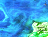
An analysis of satellite images over the area of the experiment shows that strong vortex activity took place off the northern coast of the Sambia Peninsula. This was recorded on practically daily images of MODIS Aqua and the images of ETM + Landsat-7 (3 August), OLI Landsat-8 (4 August) and MSI Sentinel-2A (7 and 10 August). Several vortex structures were identified, including at least 2 vortex dipoles, stretching along the northern coast of the Sambia Peninsula and north and northeast of the Taran Cape (Figure 12). The diameter of the cyclonic part of the larger dipole was about 30 km. Vortex dipoles, practically remaining in place, were observed on all satellite images in the visible range, from 3 August to 11 August. We can assume that these vortex structures, detected on satellite images, kept the Lagrangian drifter in the launch area for an entire week.
Our assumption is based on a statistical analysis of the results of drift-experiments, which we conducted for 5 years, from 2014 to 2018. In the absence of vortices in the Cape Taran area – and this was in 18 cases out of 20 – the drifter was left in the south-west, spreading along the western coast of the Sambian Peninsula, performing inertial oscillations (loops), or, in the case of stable eastern currents, spreading along the northern coast of the Sambian Peninsula, towards the Curonian Spit [Lavrova et al., 2018]. Only in the presence of stable vortex structures did it remained for a long time in a localized region, as we saw in August 2015.
Thus the results in the case studies show that in the coastal zone of Southeastern Baltic the surface circulation is determined not only by wind forcing but also by the presence of vortex structures in the area. This feature can play a critical point during propagation of surface pollutants forecast, in particular oil spills, commonly detected in the regions with an intensive commercial shipping. Results of drifter experiments convincingly demonstrated that in the case of submesoscale vortex structure (eddy dipoles and others) presence in the area the passive floating objects, as drifters or pollutants, propagates in a very localized area during long time intervals. In a case of a weak vortex activity pollutants will propagate over vast territory. Joint analysis of real-time data derived from remote sensing monitoring and drifter experiments allowed us to provide an operational forecast of surface pollutants propagation.
The paper describes the application of Lagrangian mini-drifters in studies of coastal ocean circulation. A comparison of the real trajectories of our mini-drifters with the predicted ones from the interactive numerical model, Seatrack WEB HELCOM, with different wind factors, showed that the propagation of drifters, described in the article, strictly coincides with a current, and the wind force has a minimal direct effect on drifters.
As shown by our experiments in the Southeastern Baltic Sea, an application of Lagrangian mini-drifters makes it possible to detect the presence of complex sub-mesoscale vortex processes and inertial oscillations, i.e., processes that are difficult to simulate numerically. Our many-year remote sensing monitoring shows [Lavrova et al., 2011] that a presence of different vortex structures in the Southeastern Baltic could strongly influence the propagation of surface pollutants and oil spills, regularly determined on satellite images. Joint analysis of remote sensing data and drifter experiments can help us improve the operational forecast of surface pollutants propagation. Case study described in the paper shows that the presence of submesoscale eddies, determined by remote sensing data influences the passive objects (drifts, oil anthropogenic pollution and so on) which are able to keep floating in a strictly localized area for at least 1 week, even in changeable wind conditions.
Despite some limitations of Lagrangian GPS/GSM drifters application (GSM coverage, GPS accuracy, grid deformation and high possibility of lost) they are very informative and affordable for researches with constrained budgets, and it is an easily accessible method of studying near-coast circulation.
A comparative analysis of data obtained from such mini-drifters and an Acoustic Doppler Current Profiler (ADCP) is based on in-situ studies of currents in the coastal part of the Black Sea. When the average current velocity is greater than 20 cm/s, an error in determining the absolute current magnitudes by two types of instruments does not exceed 3 cm/s. There are some advantages of using mini-drifters. While ADCP has a "blind zone" at depth of about 2 m, Lagrangian drifters can measure currents at this shallow depth. Drifters can also record a low flow rate of currents, which are not detected by the ADCP method. Drifters can be used to determine the flow direction at any flow rate, in contrast to ADCP, for which the flow direction is not determined if the velocities are small, for example, when it is less than 5 cm/s, which is shown in the experiment described in this paper.
The low cost of manufacturing drifters ($\sim 150$ USD per system) along with the low cost of GSM communications, the ease of manufacturing and operation, with no special technical experience required, and the link to obtaining operational data in real-time for up to several weeks make these systems valuable supplementary tools for remote sensing studies of processes in coastal zones.
Ambjörn, C., et al. (2011), Seatrack Web: The HELCOM Tool for Oil Spill Prediction and Identification of Illegal Polluters, Oil Pollution in the Baltic Sea, Kostianoy A., Lavrova O. (eds.) The Handbook of Environmental Chemistry, Vol. 27, Springer-Verlag, Berlin, Heidelberg, https://doi.org/10.1007/698_2011_120.
Blumberg, A. F., G. L. Mellor (1987), A Description of a Three-Dimensional Coastal Ocean Circulation Model, 1–16 pp., American Geophysical Union, Washington, DC, https://doi.org/10.1029/CO004p0001.
Carlson, D. F., et al. (2010), How useful are progressive vector diagrams for studying coastal ocean transport?, Limnology and Oceanography: Methods, no. 8, p. 98–106, https://doi.org/10.4319/lom.2010.8.0098.
D'Asaro, E., A. Shcherbina, et al. (2018), Ocean convergence and dispersion of flotsam, Proceedings of the National Academy of Sciences, 115, no. 6, p. 1162–1167, https://doi.org/10.1073/pnas.1718453115.
Davis, R. E. (1985), Drifter observations of coastal ocean surface currents during CODE: The statistical and dynamical views, J. Geophys. Res., 90, no. C3, p. 4756–4772, https://doi.org/10.1029/JC090iC03p04756.
Gade, M., B. Seppke, L. Dreschler-Fischer (2012), Mesoscale surface current fields in the Baltic Sea derived from multi-sensor satellite data, Intern. J. Remote Sens., 33, no. 10, p. 3122–3146, https://doi.org/10.1080/01431161.2011.628711.
Ginzburg, A., E. Bulycheva, A. Kostianoy, et al. (2015a), Vortex dynamics in the Southeastern Baltic Sea from satellite radar data, Oceanology, 55, no. 6, p. 805–813, https://doi.org/10.1134/S0001437015060065.
Ginzburg, A. I., E. V. Bulycheva, A. G. Kostianoy, D. M. Solovyev (2015b), On the role of vortices in the transport of oil pollution in the Southeastern Baltic Sea (according to satellite monitoring), Sovremennye problemy distantsionnogo zondirovaniya Zemli iz kosmosa, 12, no. 3, p. 149–157.
Hordoir, R., B. W. An, J. Haapala, H. E. M. Meier (2013), A 3d Ocean Modelling Configuration for Baltic and North Sea Exchange Analysis. Technical Report, 1–72 pp., SMHI, Norrköping (ISSN 0283-1112).
Jankowski, A. (2002), Variability of coastal waters hydrodynamics in the Southern Baltic: Hindcast modeling of upwelling event along the Polish coast, Oceanologia, 44, no. 4, p. 395–418.
Joseph, A. (2014), Measuring Ocean Currents, 1st edition, 1–430 pp., Elsevier Science B.V., Amsterdam, The Netherlands (ISBN 9780123914286).
Karimova, S., M. Gade (2016), Improved statistics of submesoscale eddies in the Baltic Sea retrieved from SAR imagery, Intern. J. Remote Sens., 37, no. 10, p. 2394–2414, https://doi.org/10.1080/01431161.2016.1145367.
Lavrova, O., M. Mityagina, T. Bocharova, M. Gade (2008), Multichannel observation of eddies and mesoscale features in coastal zones, Remote Sensing of the European Seas, Barale V. and Gade M. (eds.), p. 463–474, Springer Verlag, Berlin, https://doi.org/10.1007/978-1-4020-6772-3_35 (ISBN 978-1-4020-6771-6).
Lavrova, O., S. Karimova, M. Mityagina (2010), Eddy activity in the Baltic Sea retrieved from satellite SAR and optical data, Proceedings of 3rd Intern. Workshop SeaSAR 2010, Special Publication ESA-SP-679, p. 1–5, ESA, Frascati, Italy.
Lavrova, O. Y., A. G. Kostianoy, S. A. Lebedev, M. I. Mityagina, A. I. Ginzburg, N. A. Sheremet (2011), Complex Satellite Monitoring of the Russian Seas, 194–197 pp., IKI RAN, Moscow, Russia (ISBN 978-5-9903101-1-7).
Lavrova, O. Yu., M. I. Mityagina, A. G. Kostianoy (2016), Satellite Methods for Detecting and Monitoring Marine Zones of Ecological Risk, 1–336 pp., IKI RAN, Moscow, Russia (ISBN 978-5-00015-004-7).
Lavrova, O. Y., E. V. Krayushkin, K. R. Nazirova, A. Y. Strochkov (2018), Vortex structures in the Southeastern Baltic Sea: Satellite observations and concurrent measurements, Remote Sensing of the Ocean, Sea Ice, Coastal Waters, and Large Water Regions 2018, Proceedings Volume 10784, SPIE, Berlin, Germany, https://doi.org/10.1117/12.2325463.
LaCase, J. H. (2008), Statistics from Lagrangian observations, Progress in Oceanography, 77, p. 1–29, https://doi.org/10.1016/j.pocean.2008.02.002.
Lumpkin, R., T. Ozgokmen, L. Centurioni (2017), Advances in the application of surface drifters, Annual Review of Marine Science, no. 9, p. 59–81, https://doi.org/10.1146/annurevmarine010816-060641.
Lynch, D. R., D. A. Greenberg, et al. (2015), Particles in the Coastal Ocean: Theory and Applications, Cambridge University Press, Cambridge (ISBN 9781107061750).
Madec, G., P. Delecluse, M. Imbard, C. Levy (1998), OPA 8.1 Ocean General Circulation Model reference manual. Note du Pôle de modélisation, 1–91 pp., Institut Pierre Simon Laplace (IPSL), France.
Madec, G. (2008), NEMO Ocean Engine, User Manual, Note du Pôle de modélisation, Institut Pierre Simon Laplace (IPSL), France (ISSN 1288-1619).
Marmorino, G. O., B. Holt, Molemaker} {M. J. , P. M. DiGiacomo, M. A. Sletten (2010), Airborne synthetic aperture radar observations of "spiral eddy" slick patterns in the Southern California Bight, J. Geophysical Research, 115, no. C05010, https://doi.org/10.1029/2009JC005863.
Niiler, P. P., R. E. Davis, H. White (1987), Water-following characteristics of a mixed layer drifter, Deep-Sea Res., 34, no. 11, p. 1867–1881, https://doi.org/10.1016/0198-0149(87)90060-4.
Poulain, P.-M., R. Barbanti, et al. (2005), Statistical description of the Black Sea near surface circulation using drifters in 1993–2003, Deep-Sea Res., 52, p. 2250–2274, https://doi.org/10.1016/j.dsr.2005.08.007.
Poje, A., T. Ozgokmen, B. Lipphardt Jr., B. Haus, E. Ryan, A. Haza, et al. (2014), Submesoscale dispersion in the vicinity of the Deepwater Horizon spill, Proceedings of the National Academy of Sciences, 111, p. 12,693–12,698, https://doi.org/10.1073/pnas.1402452111.
Svendsen, E., J. Berntsen, M. Skoden, B. Adlandsvik, E. Martinsen (1996), Model simulation of the Skagerrak circulation and hydrography during Skagex, J. Mar. Syst., no. 8, p. 219–237, https://doi.org/10.1016/0924-7963(96)00007-3.
Sybrandy, A. L., P. P. Niiler (1991), WOCE/TOGA Lagrangian drifter construction manual, WOCE Report No 63; SIO Report No 91/6, Scripps Institution of Oceanography, La Jolla.
Zhurbas, V. M., I. S. Oh, V. T. Paka (2003), Generation of cyclonic eddies in the Eastern Gotland Basin of the Baltic Sea following dense water inflows: Numerical experiments, J. Mar. Syst., no. 38, p. 323–336, https://doi.org/10.1016/S0924-7963(02)00251-8.
Zhurbas, V., T. Stipa, et al. (2004), Generation of subsurface cyclonic eddies in the southeast Baltic Sea: Observations and numerical experiments, J. Geophys. Res., 109, no. C05033, https://doi.org/10.1029/2003JC002074.
Received 11 October 2018; accepted 12 November 2018; published 1 January 2019.

Citation: Krayushkin Evgeny, Olga Lavrova, Alexey Strochkov (2019), Application of GPS/GSM Lagrangian mini-drifters for coastal ocean dynamics analysis, Russ. J. Earth Sci., 19, ES1001, doi:10.2205/2018ES000642.
Copyright 2019 by the Geophysical Center RAS.