
RUSSIAN JOURNAL OF EARTH SCIENCES, VOL. 15, ES3004, doi:10.2205/2015ES000555, 2015
Azad A. Mansoori1, Parvaiz A. Khan2, Roshni Atulkar3, P. K. Purohit3, A. K. Gwal1
1Department of Electronics, Barkatullah University, Bhopal, MP, India
2Department of Electronics and Communication Engineering, Islamic University of Science and Technology, Pulwama, J&K, India
3National Institute of Technical Teachers' Training and Research, Bhopal, MP, India
.All the transionospheric signals interact with the ionosphere during their passage through ionosphere, hence are strongly influenced by the ionosphere. One of most important ionospheric effects on the transionospheric signals is the delay both in range and time. Under this investigation we have studied the variability of ionospheric range delay in GPS signals. To accomplish this study we have used the GPS measurements at a low latitude station, IISC Bangalore (13.02° N, 77.57° E) during January 2012 to December 2012. We studied the diurnal, monthly as well as seasonal variability of the range delay. We also selected five intense geomagnetic storms that occurred during 2012 and investigated the variability of delay during the disturbed conditions. From our study we found the diurnal variability of the range delay is similar to the diurnal pattern observed for the Total Electron Content (TEC). The delay is maximum during the month of October while lowest delay is found to occur in the month of December. During summer season the range delay in GPS signals is less while the largest delay occurs during the equinox season. The variability of delay during the geomagnetic storms of 09 March 2012, 24 April 2012, 15 July 2012, 01 October 2012 and 14 November 2012 were also studied. All these geomagnetic storms belonged to intense category. We found that the value of delay is strongly increased during the course of geomagnetic storms.
The GPS signals from the satellites while propagating through a disturbed ionospheric medium undergo changes in their characteristics depending on the extent of disturbance. The ionosphere is a dispersive medium, it implies that the ionosphere bends the GPS radio signal from its optical path and it happens due to change in its speed while propagating through various layers of ionosphere. A significant range error is caused by the change in the propagation speed. The ionosphere speeds up the propagation of the carrier phase, whereas it slows down the pseudo range code measurement by an equivalent amount. In other words, the GPS code information is delayed resulting in the pseudo range being measured too long as compared to the geometric distance of the satellite [Hofmann et al., 1992]. So, the receiver-satellite distance will be too short if measured by the carrier phase and is too long if measured by code as compared to the actual distance. The ionospheric time delay is directly proportional to the Total Electron Content (TEC) along the path of propagating signal between the satellite and user (1 meter for 6.15 TEC units on L1 frequency) [Klobuchar et al., 1975]. TEC is highly dependent on many variables such as local time, season, geomagnetic location and the level of solar and magnetic disturbances.
Strong ionospheric disturbances have great impact on performances of the GPS receivers. The ionospheric effects on the GPS receivers have been studied by many researchers [Doherty et al., 2000; Groves et al., 2000; Hegarty et al., 2001; Skone, 2001; Conker et al., 2003; Bhattacharya et al., 2008, 2009; Shukla et al., 2009; Jain et al., 2010]. The positional accuracy of the GPS system is limited by the precision in measuring atmospheric time delay. Precise ionospheric and tropospheric time delay estimation is required for achieving high level of accuracy in determination of position, navigation and geodesy. It is well established that estimation of precise time delay by means of monitoring the clocks on GPS satellites can be limited by the time delay of the Earth's ionosphere. At equatorial and low latitudes TEC is highly variable with local time, season and level of solar and magnetic activity. The dominant variability is diurnal due to the large variation in incident solar radiation, so the time delay is also highly variable at low latitudes. At equatorial regions, the Earth's magnetic field is horizontal and there is east-west electric field due to the dynamic effect produced by the atmospheric motions. During the day the electric field is eastward and westward during the night. This phenomenon also causes irregularity in the ionospheric condition, hence contributes to the delay mechanism.
The range obtained between the satellite and user by integrating the phase and group refractive indices along the path of GPS signal is different from the true range. The difference between measured range and the true range is known as ionospheric error. This error is negative for the carrier phase pseudo ranges and positive for the code pseudo ranges [Komjathy, 1997]. The delay due to the ionosphere results in range errors which may vary from few meters to tens of meters. The ionosphere is a dispersive medium i.e., its refractive index is a function of the operating frequency [Davies, 1966; Kaplan, 1996; Misra and Enge, 2006]. Thus appropriate methods can be adopted for determining the extent of delay due to ionosphere using code observations at L1 (1575.42 MHz) or at both L1 (1575.42 MHz) and L2 (1227.60 MHz) GPS frequencies. Typically ionospheric delay on GPS observations can be reduced by using the combination of two broadcasting frequencies, by using delay model of ionosphere for single frequency users [Kleusberg, 1998]. In recent years various ionospheric delay models were proposed [Klobuchar, 1986; Walker, 1989; Coster et al., 1992]. The effects of ionosphere on GPS performances can be considered in two aspects: first during strong ionospheric disturbances and second due to the amplitude and phase variations of GPS signals due to the disturbances. During these adverse conditions, conventional models can not accurately describe the ionospheric delay. Thus, for achieving precise GPS positioning, the ionospheric effects must be eliminated so that the more precise position could be measured. Hence ionospheric threat models are required to evaluate impact of disturbances on positioning accuracy, which is an important factor for system integrity [Luo et al., 2004].
|
| Table 1 |
To study the variability of ionospheric delay we have used the GPS observations carried out at low latitude station of India, IISC Bangalore (13.02° N, 77.57° E). For our study we have used only the data of year 2012 (January 2012 to December 2012). We also selected the five geomagnetic storms that occurred during 2012 to study variability of ionospheric delay during disturbed conditions. Only the five most intense ($Dst \leq -100$ nT) geomagnetic storms were considered for the present study. The availability of various data sets was also checked and events with bad or missing data were removed from the analysis. The complete catalogue of all the selected five events is provided in Table 1 along with various important characteristics.
To accomplish this study we have made use of three types of data sets; GPS data, $Dst$ index and IMF $B_z$. A complete network of GPS receivers has been setup worldwide since last couple of decades, and the observations are carried out regularly. The data obtained in this way is freely available to users. This service commonly known as International GPS Service (IGS) provides the data of hundreds of stations from all parts of the world. GPS navigation and observation data downloaded from the IGS centres are in compressed RINEX format. The time sampling of the data is 30 seconds. The TEC along the path from satellite to receiver, (STEC), at the two GPS frequencies, $\mathrm{L1} = \mathrm{f1} = 1.57542$ GHz and $\mathrm{L2} = \mathrm{f2} = 1.2276$ GHz, can be calculated using formula by Klobuchar, [1996].
The GPS TEC data used in this study were obtained from the IGS for the IGS station IISC Bangalore (13.02° N, 77.57° E). However, for the present analysis, the data obtained using code measurement is only used from January to December 2012 for all the days. From the processed data, elevation angle and TEC are used to estimate the time delay values at elevation cut off 40°.
The most widely used ionospheric model for estimation of ionospheric delay is the grid based ionospheric model. However we have used another model for estimation of ionospheric delay at user position. This method uses GPS pseudo-range measurements at both L1 and L2 frequencies. GPS pseudo-range and carrier phase range measurements are estimated based on assumptions that the signal velocity and wavelength are equal to those values valid for an electromagnetic wave propagating in vacuum. However, the ionospheric index of refraction has a non-unit value due to the physical properties of the ionosphere, therefore the assumption that the GPS signal travels at the speed of light in vacuum and with wavelength equal to the wavelength in vacuum is incorrect. The group velocity, however, is less than the speed of light, and causes the group delay. The phase and group velocities can be derived as follows:
\begin{eqnarray*} v_g = \frac{c}{n_g} = \frac{c}{1+\frac{40.3N}{f^2}} \approx c \left( 1-\frac{40.3N}{f^2} \right) \end{eqnarray*} \begin{eqnarray*} v_p = \frac{c}{n_p} = \frac{c}{1-\frac{40.3N}{f^2}} \approx c \left( 1+\frac{40.3N}{f^2} \right) \end{eqnarray*}The phase ionospheric range delay, $\Delta \Phi$, and the group range delay, $\Delta P$, which are caused by the phase advance and the group delay, respectively, can therefore be derived by subtracting the assumed velocity, $c$, and the true velocities ($v_p$ and $v_g$) multiplied by the travel time of the signal and can be expressed as follows:
\begin{eqnarray*} \Delta \Phi = \int\limits_{\mathrm{path}}(n_p - 1) dl = -\frac{40.3}{f^2} \int\limits_{\mathrm{path}} Ndl = \frac{40.3}{f^2} \mathrm{TEC} \end{eqnarray*} \begin{eqnarray*} \Delta P = \int\limits_{\mathrm{path}}(n_g - 1) dl = -\frac{40.3}{f^2} \int\limits_{\mathrm{path}} Ndl = \frac{40.3}{f^2} \mathrm{TEC} \end{eqnarray*}The magnitude of the range errors is equal for both carrier phase and pseudo range measurements but with the opposite sign. The quantity $\int_{\mathrm{path}} Ndl$ can be evaluated by integrating electron density along the signal path. This quantity represents Total Electron Content (TEC). The Total Electron Content is computed and converted into ionospheric delay in meters using a conversion factor. Following relation has been used to get the total ionospheric delay (including receiver bias and P1–P2 bias):
\begin{eqnarray*} \mathrm{TEC}=9.483 \left(R_{\mathrm{L2}}-R_{\mathrm{L1}}\right) - \mathrm{TEC}_{\mathrm{RC}} - \mathrm{TEC}_{\textrm{P1–P2}} \end{eqnarray*}where $R_{\mathrm{L1}}$ is pseudo range at L1 frequency; $R_{\mathrm{L2}}$ is pseudo range at L2 frequency; $\mathrm{TEC_{RC}}$ is receiver bias error/0.351; and $\mathrm{TEC}_{\textrm{P1–P2}}$ is P1–P2 bias error/0.351, respectively.
Therefore, the total ionospheric delay in meters is given as:
\begin{eqnarray*} \Delta I = 0.163 \mathrm{TEC} \end{eqnarray*}Since the delay due to ionosphere is one of the most important sources of error, in our analysis this delay has been estimated using GPS code observables and methods using TEC values. Ionospheric correction terms from both the methods are applied to the corresponding pseudo ranges and user position is estimated. For our investigation we have used the GPS data of the IISC Bangalore (13.02° N, 77.57° E), India downloaded from the URL http://sopac.ucsd.edu/dataBrowser.shtml.
 |
| Figure 1 |
The ionospheric conditions and so the delay changes from hour to hour, day to day, season to season as well as during disturbed and quiet solar and geomagnetic conditions. Therefore, we have studied the variability of ionospheric delay diurnally, monthly as well as seasonally. At the same we have also selected five intense geomagnetic storms and studied the variability during the disturbed geomagnetic conditions as well as compared these with the quiet conditions. The interplanetary, solar wind and geomagnetic conditions during the year 2012 are shown in Figure 1. The Figure 1 shows the variation of $Dst$ index, $Kp$ index, IMF $B_z$, Solar wind temperature, solar velocity and solar wind density for the year 2012. From the Figure 1 we clearly notice that there has been a mixed type of activity during the year 2012. There were a number of geomagnetic storms, some of them intense. Also there were large number of days for which the geomagnetic activity was quite low.
 |
| Figure 2 |
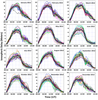
The diurnal variation of ionospheric delay for all the days of each of the twelve months of year 2012 is shown in Figure 2 for IISC Bangalore (13.02° N, 77.57° E), India. It can clearly be observed from the Figure 2 that the ionospheric delay follows a diurnal pattern similar to that of TEC. It starts increasing in the morning of each day and achieves peak around 0600 to 1200 hrs UT during all months of the year 2012. The delay observed highest peaks during the months of April, September and October with peak delay of about 14 meters while the shallow peaks were observed during the month of June, July, December, January and February with peak delay of about 8 meters. The diurnal pattern observed during all the months has same shape with occurrence of diurnal peak between the same times. The peak values during different days of each month vary only within in range of about 4 meters. However, the peak value changes from month to month.
 |
| Figure 3 |
The month to month variability of the ionospheric delay for each month of year 2012 at IISC Bangalore is shown in Figure 3. The variability during all the days of each month is averaged to construct the Figure 3.
The Figure 3 shows that the monthly variation of ionospheric delay is maximum during the month of October and reaches a maximum of 6 meters while the minimum delay is observed during the month of December with maximum value of 3.6 meters. The ionospheric delay starts increasing from the month of December and achieves peak in the month of March after that it again starts decreasing and reaches minimum in the month June or July. Then it starts increasing again and reaches maximum during the month of October after which it starts decreasing and by the end of December it reaches to minimum for the start of next cycle. Therefore, we see that monthly variability of ionospheric delay follows a semi-annual type of variability.
We have also studied the seasonal variability of ionospheric delay at IISC Bangalore. The seasonal variability of ionospheric delay during three different seasons of the year 2012 at IISC Bangalore is shown in Figure 3. This figure shows that the ionospheric delay is maximum during the equinox season with maximum value of 5.5 meters while the minimum delay is observed during the summer season with maximum delay 4.2 meters.
The disturbed and adverse geomagnetic conditions have a significant impact on the ionosphere. Consequently, the ionospheric delay is also expected to be significantly affected by the adverse geomagnetic conditions. To investigate the variability of ionospheric delay during disturbed geomagnetic conditions we have selected five most intense geomagnetic storms of year 2012. The geomagnetic storms of 09 March 2012, 24 April 2012, 15 July 2012, 01 October 2012 and 14 November 2012 were selected to study the behaviour of ionospheric delay during these geomagnetic storm conditions. All the five cases are discussed serially as follows.
 |
| Figure 4 |
One of the intense geomagnetic storms of year 2012 was observed on 09 March 2012. The storm had a sudden commencement phase followed by the initial and main phase. The storm intensity index $Dst$ had the minimum or peak value of $-143$ nT. The recovery phase of the storm lasted for a couple of days after the main phase. Prior to the onset of this geomagnetic storm the $z$ component of Interplanetary Magnetic Field (IMF) $Bz$ was in southward direction for a substantial period of time and achieved a peak value of $-17$ nT. The solar wind conditions were also above their normal values. These conditions were responsible for the geomagnetic storm of 09 March 2012. The behaviour of ionospheric delay before, after and on the storm day along with $Dst$ index and IMF $B_z$ index are shown in Figure 4. From this figure we see that on the day of geomagnetic storm main phase i.e. 09 March 2012 the ionospheric delay is larger than on 08 March and 10 March. The ionospheric delay on 09 March was 12 meters while on 08 and 10 March the delay was 10.5 and 10 meters, respectively. The enhancement on the storm day in the ionospheric delay is 1.8 meters from the median of the March month. Thus the impact of geomagnetic storm is clearly seen on the ionospheric delay as a positive enhancement.
 |
| Figure 5 |
An intense storm of year was observed on 24 April 2012. The minimum $Dst$ recorded during this storm was $-104$ nT. The most important factor responsible for a geomagnetic storm is the south directed IMF $B_z$. We also observed a southward turning of IMF $B_z$ prior to the onset of the geomagnetic storm with a peak value $-16$ nT. The effect of this geomagnetic storm on the ionospheric delay is shown in Figure 5 along with changes in storm intensity index $Dst$ and IMF $B_z$. The main phase of the geomagnetic storm was observed on 24 April 2012, but the effect of this storm was observed on the other day i.e. 25 April 2012. The maximum delay observed on 25 April 2012 was 13.2 meters while on 24 April and 26 April the delay was 10.8 meters and 11 meters respectively. An enhancement of 2.9 meters from the median of the month was observed during this storm. Hence during this storm we also observed a positive but delay effect.
 |
| Figure 6 |
The effect of geomagnetic storm of 15 July 2012 on the ionospheric delay is shown in Figure 6. The geomagnetic storm that occurred on 15 July 2012 was an intense geomagnetic storm with peak or minimum $Dst$ $-133$ nT. The peak value of IMF $B_z$ prior to the onset of this geomagnetic was $-20$ nT. The effect of this storm on the ionospheric delay was very strong. The peak value of the ionospheric delay on the day of main phase of geomagnetic storm, 15 July 2012, was 10.5 meters while the peak values of ionospheric delay on 14 July and 16 July 2012 was 6.2 and 6.3 meters respectively. The enhancement in the ionospheric delay from the median of the month was recorded as 3.2 meters.
4.4.4. Case 4: 01 October 2012.
 |
| Figure 7 |
The geomagnetic storm of 01 October 2012 has the same minimum $Dst$ as the storm of 15 July 2012. Both the geomagnetic storms had the minimum or peak $Dst$ as $-133$ nT as well as the same IMF $B_z$ peak i.e. $-20$ nT. However the effect of both the storms on the ionospheric delay was different. The effect of geomagnetic storms of 01 October 2012 on the ionospheric delay is shown in Figure 7. The peak ionospheric delay on 01 October 2012 was 12.37 meters while as the delay on 30 September 2012 and 02 October 2012 was 11 and 10.6 meters respectively. The enhancement in the ionospheric delay form the median of the month during this storm was observed as 1.79 meters which is almost half of the enhancement observed during the storm of 15 July 2012. Thus we find that even the geomagnetic storms of same intensity do not produce the same effect on the ionospheric delay.
4.4.5. Case 5: 14 November 2012.
 |
| Figure 8 |
The effect of geomagnetic storm of 14 November 2012 on the ionospheric delay is shown in Figure 8. The minimum $Dst$ of this geomagnetic storm was $-109$ nT. The minimum IMF $B_z$ prior to the onset of this geomagnetic storm was $-18$ nT. The ionospheric delay observed on the day of main phase of storm i.e. 14 November 2012 was 12.31 meters while the delay on the two control days i.e. 13 November 2012 and 15 November 2012 was 11.2 and 11.9 meters. The enhancement in the ionospheric delay from the median of the month was recorded as 3.33 meters. This is the strongest enhancement among all the selected events. Although, the intensity of this geomagnetic storm was not too large like other storms but the effect on ionospheric delay was the strongest. It shows that the storm of any intensity can produce a significant impact on the ionospheric delay.
 |
| Figure 9 |
We then constructed the diurnal profile of the ionospheric delay during all the five storms events and then compared these with the two control days and median of the month. The diurnal profile of ionospheric delay on the storm day, control days and median day during all the selected five storm events are shown in Figure 9.
The profile on the storm day is shown by the red color, the profile on two control days are shown by wine and blue while the profile of the median of month is shown by olive color. We found that during the storm events the profile of ionospheric delay is above the profile of two control days as well as median of the month. However, in case of the 24 April 2012 storm event we notice that profile on the storm day is below the control days and median of the month. This is due to reason that during this storm the post effect was observed. The storm effect was not observed on the storm day but the next day i.e. 25 April 2012. Therefore, we have also plotted the profile of another day i.e. 26 April 2012. Therefore, we clearly notice that all the geomagnetic storms produce a positive significant effect on the ionospheric delay either on the storm day or after the storm day.
The main conclusions of the study are enumerated below:
Bhattacharya, S., P. K. Purohit, A. K. Gwal (2009), Ionospheric time delay variations in the equatorial anomaly region during low solar activity using GPS, Indian J. Radio Space, 38, no. 5, p. 266–274.
Conker, R. S., M. B. El-Arini, C. J. Hegarty, T. Hsiao (2003), Modelling the effects of ionospheric scintillation on GPS/satellite based augmentation system availability, Radio Science, 31, no. 1, p. 1-1–1-23, doi:10.1029/2000RS002604.
Coster, A. J., E. M. Gaposchkin, L. E. Thornton (1992), Real-time ionospheric monitoring system using GPS, J. Inst. Navig., 39, no. 2, p. 191–204, doi:10.1002/j.2161-4296.1992.tb01874.x.
Davies, K. (1966), Ionospheric radio propagation, Dover Publications Inc., New York.
Doherty, P. H., S. Delay, C. Valladares, J. Klobuchar (2000), Ionospheric scintillation effects in the equatorial and auroral region, Proceedings of ION-GPS 2000, The Institute of Navigation, Salt Lake City, Utah.
Groves, K., S. Basu, J. M. Quinn, T. R. Pedersen, K. Falinski (2000), A comparison of GPS performance in scintillation environment at Ascension Island, Proceedings of ION-GPS 2000, The Institute of Navigation, Salt Lake City, Utah.
Hegarty, C., M. El-Arini, T. Kim, S. Ericson (2003), Scintillation modeling of GPS wide area augmentation system receivers, Radio Science, 36, no. 5, p. 1221–1232, doi:10.1029/1999RS002425.
Hofmann-Wellenhof, B., H. Lichtenegger, J. Collins (1992), Global Positioning System: Theory and Practice, 4th edition, 390 pp., Springer-Verlag, Wien, doi:10.1007/978-3-7091-5126-6.
Jain, A., S. Tiwari, S. Jain, A. K. Gwal (2010), TEC response during severe geomagnetic storms near the crest of equatorial ionization anomaly, Indian J. Radio Space, 39, no. 1, p. 11–24.
Kaplan, E. D. (1996), Understanding GPS: Principles and Applications, 554 pp., Artech House, Norwood, MA.
Kleusberg, A. (1998), Atmospheric models from GPS, GPS for geodesy, 2nd edition, edited by P. Teunissen, p. 599–623, Springer, Wien.
Klobuchar, J. A. (1975), Polarization of VHF waves emitted from geostationary satellites, J. Geophys. Res., 80, no. 31, p. 4387–4389, doi:10.1029/JA080i031p04387.
Klobuchar, J. A. (1986), Design and Characteristics of the GPS ionospheric time delay algorithm for single frequency users, Proceedings of the PLANS-86 conference, New York, Institute of Electrical and Electronic Engineers, Las Vegas, NV.
Klobuchar, J. A. (1996), Ionospheric Effects on GPS, Global Positioning System: Theory and Applications, Volume I, edited by B. W. Parkinson and J. J. Spilker, p. 485–515, American Institute of Aeronautics and Astronautics, Washington, DC.
Komjathy, A. (1997), Global Ionospheric Total Electron Content Mapping Using the Global Positioning System, Ph.D. dissertation, Department of Geodesy and Geomatics Engineering Technical Report No. 188, University of New Brunswick, Fredericton, New Brunswick, Canada.
Luo, M., S. Pullen, A. Ene, D. Qiu, T. Waller, P. Enge (2004), Ionosphere threat to LAAS: Updated model, user impact and mitigations, Proceedings of ION-GNSS 2004, The Institute of Navigation, Long Beach, CA.
Misra, P., P. Enge (2006), Global Positioning System: Signals, Measurements and Performance, 2nd edition, 569 pp., Ganga Jamuna Press, Massachusetts.
Shukla, A. K., P. Shinghal, M. Sivaraman, K. Bandyopadhyay (2009), Comparative analysis of the effect of ionospheric delay on user position accuracy using single and dual frequency GPS receivers over Indian region, Indian J. Radio Space, 38, no. 1, p. 57–61.
Skone, S. H. (2001), The impact of magnetic storm on GPS receiver performance, J. Geodyn., 75, no. 6, p. 457–472, doi:10.1007/s001900100198.
Walker, J. K. (1989), Spherical cap harmonic modeling of high latitude magnetic activity and equivalent sources with sparse observations, J. Atmos. Terr. Phys., 51, no. 2, p. 67–80, doi:10.1016/0021-9169(89)90106-2.
Received 26 July 2015; accepted 4 September 2015; published 22 October 2015.

Citation: Mansoori Azad A., Parvaiz A. Khan, Roshni Atulkar, P. K. Purohit, A. K. Gwal (2015), Ionospheric influences on GPS signals in terms of range delay, Russ. J. Earth Sci., 15, ES3004, doi:10.2205/2015ES000555.
Copyright 2015 by the Geophysical Center RAS.