
RUSSIAN JOURNAL OF EARTH SCIENCES, VOL. 15, ES3002, doi:10.2205/2015ES000553, 2015
Hong-Chun Wu1, Ivan N. Tikhonov2, Ariel R. Césped3
1Institute of Labor, Occupational Safety and Health, Taipei, Taiwan
2Institute of Marine Geology and Geophysics of FEB RAS, Yuzhno-Sakhalinsk, Russia
3Department of Mechanic Engineering, University of Santiago, Santiago, Chile
.[1] Many scientists around the world have reported the occurrence of atmospheric anomalies prior to earthquakes. According to the Lithosphere-Atmosphere-Ionosphere Coupling (LAIC) model, the thermal flux results in temperature rising, humidity and pressure drop, and finally, changes in the velocity line when jet-stream passes through the region over the future epicenter. Using satellite observation, we tried to find out the possible atmospheric disturbances in the surface latent heat flux (SHLF), meteorological features, and jet-stream velocity change before the powerful $M =7.8$ Nepal Earthquake on 25 April 2015 and $M= 6.6$ Taiwan Earthquake on 20 April 2015. To reinforce these observations, a numerical modeling of seismology regime dynamics is also performed.
Geological faults have defined cycles of activity, with an associated accumulation of energy due to shear generated at the crustal region. The process before distension and rupture (usually followed by an earthquake) shows physical phenomena that have been described as seismic precursors Freund, 2009] suggests that rocks under high mechanical pressure emit vacuum ions (p-holes) cluttering the air. On the other hand, the crustal regions prepared for an earthquake release radioactive elements such as radon (222Rn), and their decay produces radicals in the air. Be that as it may, the final result is a thermodynamically unstable state, favoring a process of phase change due to nucleation of water and the formation of aerosols, impacting significantly the psychrometry of the a releasing latent heat in the process according to the models of free energy [Dey and Singh, 2003; Saradjian and Akhoondzadeh, 2011; Zhang et al., 2013] and generating convective processes in the troposphere. The thermal flux results in temperature rising, a drop in the humidity and pressure, and finally, changes in the velocity line when jet-stream passes through the region over the future epicenter [Ouzounov et al., 2010; Pulinets and Ouzounov, 2011]. A jet-stream is a rapidly flowing narrow air stream with almost horizontal axis in upper troposphere or low stratosphere. The dimension of the jet-streams is determined according to wind speed contour (isotach) of 108 km/h (30 m/s). As usual, the length of jet streams is several thousand kilometers, its width could be hundreds of kilometers and thickness is around 4–5 km. Simultaneous analysis of the jet-stream maps and earthquake data of $M > 6.0$ have been made [Wu and Tikhonov, 2014a].
It has been found that interruption or velocity flow lines cross above an epicenter of earthquake take place 1–70 days prior to event. The duration of this phenomenon was 6–12 hours. The average distance between epicenters and jet-stream's precursor was about 36.5 km. The forecast during 30 days before the earthquake was 66.1% [Wu and Tikhonov, 2014a]. This technique has been used to predict the strong earthquake and pre-registered on the website. There was satisfactory accuracy of the epicenter location, and the short alarm period [Wu and Tikhonov, 2014a, 2014b]. In addition, a numerical modeling of seismic regime dynamics (weak seismic events flux) is used [Malyshev and Tikhonov, 1991, 1996, 2007] to support the observations. Using satellite observation, we tried to find out the possible atmospheric disturbances for the surface latent heat flux, meteorological features, and jet stream velocity changes before the powerful $M= 7.8$ Nepal Earthquake on 25 April 2015 and $M= 6.6$ Taiwan Earthquake on 20 April 2015, and estimated the major earthquake time by the numerical modeling of seismic regime dynamics.
The appearance of SHLF usually occurs on large scale in areas next to faults. Dr. Dobrovolsky proposes an empirical relationship between the dimension of thermal/electromagnetic precursors and eventual magnitude of earthquakes [Dobrovolsky, 1991]:
\begin{equation} \tag*{(1)} \rho = 10^{0.43 M} \end{equation}
Therefore, the extent of surface latent heat flux (SHLF) is the indicator for $M6+$ earthquakes (about 350 km) and can be detected from space by satellite. The National Center for Environment Prediction (NCEP) from the National Oceanic and Atmospheric Administration (NOAA) provides global maps of SHLF with a spatial resolution of $1 \times 1$ degrees. These include areas where latent heat flux is significant, by showing contour lines. Observation of SHLF in areas close to the epicenters is performed some days prior to earthquakes. It is noted that tropical storms, typhoons, and hurricanes have large latent heat flux; a contrast with radar maps is used to discard positive false alarms.
Climatological data related to the ion-induced nucleation (IIN) phenomena is extracted from the closest meteorological stations to the epicenter, and the anomaly index is calculated according to equation:
\begin{eqnarray*} \mbox{Anomaly index} = \frac{x_{\rm daily} - \bar{x}}{\sigma} \end{eqnarray*}where $x_{\rm daily}$ is the daily weather parameter, and both, $\bar{x}$ and $\sigma$ are the mean and standard deviation of the dataset respectively. The anomalies are shown as a drop in the trend, usually coinciding the date of the thermal flux appearance.
The meteorological maps of jet-streams at 300 mb provided by the California Regional Weather server and the data of the U.S. Geological Survey/National Earthquake Information Center (USGS/NEIC) were used. The analysis is performed as follows: (1) Find the jet-stream uniform velocity streamline brake-up, or observe if jet-stream stays at the point for a certain time on 300 mb satellite maps. (2) Check whether the disruption in the front top of jet stream is located on a fault or not. If the location of objective is on the fault, the earthquakes may occur. (3) Add a report on the web.
The last version of software for numerical modeling of seismic regime dynamics (weak seismic events flux) is used [Malyshev and Tikhonov, 2007]. The technique is based on mathematical model of foreshock sequence with the help of the following differential equation:
\begin{eqnarray*} \frac{d^2 N}{dt^2} = k \left | \frac{dN}{dt} \right |^\alpha \end{eqnarray*}where $N$ is a parameter of process (a cumulative sum of the number of shocks), and $k$, $\alpha$, are empirical constants.
A solution of this equation for any given observed earthquake sequence before a strong shock defines a vertical asymptote, which can be the most likely estimate for origin time ($T_0$) of the future main event. Satisfactory estimations of the $T_0$ parameter for large earthquakes with $M \geq 7.5$ were obtained with the help of this technique from a retrospective short-term prediction in the Kurile Islands, the Japan region and other seismic areas [Malyshev and Tikhonov, 1991, 1996, 2007]. The seismicity of the Nepal region was tested from January 1990, and the Taiwan region was tested from January 2000. We used the USGS/NEIC earthquake catalog of $M \geq 4.5$. The catalog is apparently complete for $M \geq 4.5$ events. The seismicity inside a circle of 300-km radius of epicenter was analyzed.
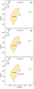
|
| Figure 1 |
The following sequence in Figure 1 shows the behavior of the SHLF in days previous of the 25 April 2015, $Mw= 7.8$ earthquake in Nepal. A 400 W/m$^2$ thermal flux in the vicinity of the epicenter was detected on 23 April 2015, two days before the main shock.
 |
| Table 1 |
Table 1 shows the results of the predicted magnitude based on Dobrovolsky's equation and actual magnitude of the studied earthquakes.
 |
| Table 2 |
Table 2 shows the distance between meteorological stations and the actual epicenter of the studied earthquakes, including the occurrence time of the psychrometric anomalies.
 |
| Figure 2 |
The next sequence (Figure 2) shows the behavior of the SHLF in days previous of the 20 April 2015, $Mw =6.6$ earthquake in Taiwan. A large 400 W/m$^2$ spot was also detected in the vicinity of the epicenter on 12 April 2015, eight days before the main shock. A record of this prediction was posted in the web [https://goo.gl/R1P1D2].
 |
| Figure 3 |
Figure 3 shows a negative anomaly (decrease) of the dew point temperature and relative humidity at the Kathmandu weather station on 23 April 2015, two days before the $M=7.8$ earthquake in Nepal.
 |
| Figure 4 |
Figure 4 shows a negative anomaly (decrease) of the dew point temperature and relative humidity at the Taipei weather station on 13 April 2015, seven days before the $M=6.6$ earthquake in northern Taiwan.
 |
| Figure 5 |
In the analysis of the jet-streams, some anomalies around the epicenter of the powerful $M=7.8$ earthquake in Nepal were detected on March 30, 2015 at 18:00 UTC; the tail end of jet-stream stayed in the area until 31 March 2015 at 00:00 UTC (Figure 5). The duration time was 6 hours. It fits the types 1 and 2 of jet-stream related to epicenter in the evaluation procedure [Wu and Tikhonov, 2014a].
 |
| Figure 6 |
In the second case, the jet-stream was interrupted to one point on 12 April 2015 at 12:00 UTC, 8 days prior to the major $M=6.6$ earthquake in Taiwan (Figure 6). This anomaly occurred near to the actual epicenter. It fits the type 2 of jet-stream related to epicenter in the evaluation procedure [Wu and Tikhonov, 2014a]. A record of this prediction was posted in the web:
$M6.6 EQ$ predicted data:
2015/04/12 2015/05/12 (24.5° N 121.8° E) $M>5.0$ 100% posted on 2015/04/14
Actual data:
$M6.6$ 2015-04-20 01:42:58 (24.129° N 122.335° E) 28.9 km [https://goo.gl/1Gjf5W]
 |
| Figure 7 |
In the results of the numerical modeling of seismology regime dynamics a non-stationary temporary behavior of the $N$ parameter is observed, i.e. the increasing in its velocity (Figure 7). The red curve is obtained as a result of modeling with the algorithm. The parameters $ k = 5.082$, $\alpha = 2.647$. The vertical asymptote indicates, on the $X$ axis, estimation of occurrence time of the powerful $M=7.8$ earthquake in Nepal (estimation corresponds to 2015/04/25 at 07:33 UTC). The difference between the estimate and the actual value of the origin time ($\Delta T$) is equal to 0.057 day.
 |
| Figure 8 |
In the second case, a non-stationary temporary behavior of the N parameter is observed, i.e. the increasing in its velocity (Figure 8). The red curve is obtained as a result of modeling with the algorithm. The parameters $k = 3.463$, $\alpha = 3.557$. The vertical asymptote indicates, on the $X$ axis, estimation of occurrence time of the major $M=6.6$ earthquake in Taiwan on 20 April 2015 (estimation corresponds to 2015/04/20 at 17:37 UTC). The forecast error of the origin time of main event is equal to 0.663 day.
According to the LAIC method [Pulinets and Ouzounov, 2011], the thermal flux as earthquake precursor might be related to air temperature increase, and humidity and pressure drop in the atmosphere. The results suggest a close relationship between the occurrence of latent heat flows and psychrometric anomalies around fault zones prior to earthquakes, highly reflected in the coincidence of occurrence time of both precursors. It seems to drive also a change in the velocity line when jet-stream passes through epicenter region [Wu and Tikhonov, 2014a]. A SHLF anomaly was detected 7 days prior to the 20 April 2015 $M=6.6$ Taiwan earthquake, while the jet-stream precursor was 8 days. However, in the case of the 25 April 2015 $M=7.8$ Nepal earthquake, the surface latent heat flux anomaly occurred 2 days before, and the jet-streams precursor was 27 days. The little time difference in the first case suggests a stronger relationship between thermal flux and stratospheric anomalies as precursors in the coastal earthquakes than continental ones. The presence of hygroscopic particles, such as salty air in undersea earthquakes could be the main factor of this phenomenon, acting as an amplifier source of the ionizing radiation. In other hand, the numerical modeling of seismic regime dynamics is not affected by this kind of environmental effects, being sensitive only by the quality of the catalogues [Malyshev and Tikhonov, 2007]. Modeling results show that a prediction error of occurrence time of great events does not exceed the first day for retroactive case of calculation. Of course, for calculation in real time errors will be much greater.
Dey, S., R. P. Singh (2003), Surface latent heat flux as an earthquake precursor, Natural Hazards and Earth System Science, 3, no. 6, p. 749–755, doi:10.5194/nhess-3-749-2003.
Dobrovolsky, I. P. (1991), The Theory of Tectonic Earthquake Preparation (in Russian), 217 pp., IPE RAS, Moscow.
Freund, F. T. (2009), Stress-Activated Positive Hole Charge Carriers in Rocks and the Generation of Pre-earthquake Signals, Electromagnetic Phenomena Associated with Earthquakes and Volcanoes, M. Hayakawa (ed.), 41–96 pp., Research Signpost, India.
Malyshev, A. I., I. N. Tikhonov (1991), Regularities in dynamics of foreshock-aftershock sequences of earthquakes around the Southern Kurile Islands, Doklady AN SSSR, 319, no. 1, p. 134–137.
Malyshev, A. I., I. N. Tikhonov (1996), Patterns of Japan Seismicity before the Large Earthquakes of 1985–1988, Russian Journal of Volcanology and Seismology, 18, p. 299–314.
Malyshev, A. I., I. N. Tikhonov (2007), Nonlinear regular features in the development of the seismic process in time, Izvestiya-Physics of the Solid Earth, 43, no. 6, p. 476–489, doi:10.1134/S1069351307060067.
Ouzounov, D., S. Pulinets, J. Y. Liu, K. Hattori, M. Parrot, M. Kafatos, T. F. Yang, H. Jhuang, P. Taylor, K. Ohyama, S. #x81;#x81;on (2010), Multidisciplinary Approach for Earthquake Atmospheric Precursors Validation by Joint Satellite and Ground Based Observations, 2010 AGU Fall meeting, p. NH24A-08, AGU, San Francisco, Calif.
Pulinets, S., D. Ouzounov (2011), Lithosphere-atmosphere-ionosphere coupling (LAIC) model – an unified concept for earthquake precursors validation, Journal of Asian Earth Sciences, 41, p. 371–382, doi:10.1016/j.jseaes.2010.03.005.
Pulinets, S., D. Ouzounov, L. Ciraolo, R. Singh, G. Cervone, A. #x81;#x81;eyva, M. Dunajecka, A. V. Karelin, K. A. Boyarchuk, A. #x81;#x81;otsarenko (2006), Thermal, atmospheric and ionospheric anomalies around the time of the Colima $M=7.8$ earthquake of 21 January 2003, Ann. Geophys., 24, p. 835–849, doi:10.5194/angeo-24-835-2006.
Saradjian, M. R., M. Akhoondzadeh (2011), Thermal detection anomalies before strong earthquakes ($M > 6.0$) using interquartile, Kalman filter and wavelet methods, Natural Hazards Earth System Sciences, 11, p. 1099–1108, doi:10.5194/nhess-11-1099-2011.
Wu, H. C., I. N. Tikhonov (2014a), Jet streams anomalies as possible short-term precursors of earthquakes with $M > 6.0$, Research in Geophysics, Special Issue on Earthquake Precursors, 4, no. 1, p. 12–18, doi:10.4081/rg.2014.4939.
Wu, H. C., I. N. Tikhonov (2014b), The Earthquake Prediction Experiment on the Basis of the Jet Stream's Precursor, 2014 AGU Fall meeting, p. NH31A-3844, AGU, Washington, DC.
Zhang, W., J. Zhao, W. Wang, H. Ren, L. Chen, G. Yan (2013), A Preliminary evaluation of surface latent heat flux as an earthquake precursor, Natural Hazards Earth System Sciences, 13, p. 2639–2647, doi:10.5194/nhess-13-2639-2013.
Received 10 August 2015; accepted 17 August 2015; published 8 September 2015.

Citation: Wu Hong-Chun, Ivan N. Tikhonov, Ariel R. Césped (2015), Multi-parametric analysis of earthquake precursors, Russ. J. Earth Sci., 15, ES3002, doi:10.2205/2015ES000553.
Copyright 2015 by the Geophysical Center RAS.