RUSSIAN JOURNAL OF EARTH SCIENCES, VOL. 13, ES1001, doi:10.2205/2013ES000526, 2013
M. Yu. Reshetnyak
Schmidt Institute of Physics of the Earth of the Russian Academy of Sciences, Moscow, Russia
.The 3D geodynamo model in the rapidly rotating spherical shell with heating from below is considered. We show that correlation of the geomagnetic dipole with total magnetic energy in the core depends on the forces balance in the dynamo system. As a result, reversals of the field not always reflect essential changes of the magnetic energy in the core. This result is closely related to the slow decay of the magnetic spectrum at the surface of the core, and in the bulk of the liquid core, especially.
The mentioned below system of geodynamo equations in the rapidly rotating spherical shell with heating from below with small variations was used from the middle ninetieth of the previous century [Jones, 2000], [Schubert, 2007]. After it was recognized that motions of the heating conductive fluid in the spherical shell can produce the magnetic field of the strength comparable with observations [Glatzmaier and Roberts, 1995], [Kuang and Bloxham, 1997], the main aim of geodynamo studies is optimization of the models and suiting results to observations.
The particular problem, which stands before geodynamo community is a modelling of the reversals and excursions of the geomagnetic field. From the point of view of the observer at the surface of the planet such events are of the great importance. At the same moment, extrapolation of the magnetic field to the surface of the liquid core decreases relative strength of the dipole mode [Langel, 1987], making it comparable with amplitude of higher harmonics, what is supported by simulations with realistic parameters [Roberts and Glatzmaier, 2000]. Moreover, analysis of the kinetic and magnetic energies spectra in the models with the quite small heat sources revealed maxima located at the high wavenumbers [Kutzner and Christensen, 2002]. As a result, the role of the dipole magnetic field in the processes in the liquid core should be reconsidered. Contribution of the dipole field into interaction of the liquid core with the solid core was also re-analyzed. In spite of the fact that volume of the inner core is 22 times smaller than of the liquid one, for years its importance for the reversal's process was indubitable. Therefore the mean-field dynamo models [Hollerbach and Jones, 1993] with the axis-symmetrical dipole magnetic field revealed deep penetration of the dipole field into the solid core, which damped too rapid reversals. However the further 3D models demonstrated small contribution of the dipole field to the total magnetic field at the inner core boundary, therefore reversals statistics did not depend on the inner core [Wicht, 2002]. Following these arguments we conclude that significance of the liquid and solid core interactions in the mean-field models was overestimated as well. In other words, importance of the geomagnetic field reversals for the processes in the bulk of the liquid core dynamo is not so obvious as it was previously supposed in geomagnetism [Jacobs, 1994]. To study this problem we consider the various scenarios of the geomagnetic field reversals in 3D dynamo model and compare our results with the most popular paleomagnetic characteristics of the field. Using numerical models with a various spatial-temporal resolution we demonstrate that variations of the force balance in the liquid core controlled by the angular velocity of the daily rotation of the planet and electrical conductivity, change the behavior of the magnetic field evolution and its spectra. This leads to the change of correlation between the dipole component and the total magnetic field energy in the liquid core.
The dynamo process driven by the flows of incompressible fluid ($\nabla\cdot {\boldsymbol{\rm V}}=0$) in a spherical shell $(r_i< r< r_0)$ rotating with the angular velocity $\Omega$ is described by the Navier-Stokes equation in the Boussinesq approximation
\begin{equation} \tag*{(1)}\label{1} {\rm E {\rm Pr}^{-1}}\left( {\partial{\boldsymbol{\rm V}}\over\partial t}+\left({\boldsymbol{\rm V}}\cdot\nabla\right){\boldsymbol{\rm V}}\right) = -\nabla P+ {\boldsymbol{\rm F}}+ {\rm E}\nabla^2{\boldsymbol{\rm V}} \end{equation}and the heat-flux equation
\begin{equation} \tag*{(2)}\label{2} {\partial T\over\partial t}+\left({\boldsymbol{\rm V}}\cdot\nabla \right) T= {\rm q}\nabla^2T. \end{equation}The magnetic field generation in the spherical shell is governed by the induction equation
\begin{equation} \tag*{(3)}\label{3} {\partial{\boldsymbol{\rm B}}\over\partial t}=\nabla\times\left({\boldsymbol{\rm V}}\times{\boldsymbol{\rm B}}\right) + \nabla^2{\boldsymbol{\rm B}}. \end{equation}The equations are scaled with the radius $L$ of a sphere as the fundamental length scale, which gives the dimensionless radius $r_o = 1$, the inner core radius $r_i$ is equal to 0.35, similar to that one of the Earth. The velocity ${\boldsymbol{\rm V}}$, pressure $P$ and time $t$ are measured in units of $\eta/L$, $\rho\eta^2/L^2$ and $L^2/\eta$ respectively, where $\eta$ is magnetic diffusivity, $\rho$ is density, $\mu$ permeability, ${\rm E} = \nu/2\Omega L^2$ is the Ekman number, $\nu$ is kinematic viscosity. The force ${\boldsymbol{\rm F}}$ includes the Coriolis, Archimedean and Lorentz forces: $ {\boldsymbol{\rm F}}= -{\boldsymbol{\rm 1}}_z\times{\boldsymbol{\rm V}}+{\rm q} {\rm Ra} Tr{\boldsymbol{\rm 1}}_r + \left(\nabla\times{\boldsymbol{\rm B}}\right)\times{\boldsymbol{\rm B}}, $ where $(r,\,\theta,\,\varphi)$ is a spherical coordinate system, ${\boldsymbol{\rm 1}}_z$ is the unit vector along the axis of rotation and ${\rm Ra} =\alpha g_o\delta T L/{ 2\Omega\kappa}$ is the modified Rayleigh number, $\alpha$ is the coefficient of volume expansion, $\delta T$ is the temperature drop through the shell, $g_o$ is the gravity acceleration at $r=r_0$, and $q=\kappa/\eta$ is the Roberts number. Eqs((1)–(3)) are closed by non-penetrating and no-slip boundary conditions for the velocity field at the rigid surfaces, constant temperature $T_i=1$ and $T_0=0$ at the inner and outer boundaries of the shell, and the vacuum boundary conditions for the magnetic field at the both boundaries. The reasons why the vacuum boundary conditions are relevant to the geodynamo problem are discussed already in introduction.
To solve Eqs((1)–(3)) we used the standard spherical functions decomposition accompanied by the poloidal-toroidal decomposition of the vector fields ${\boldsymbol{\rm V}}$ and ${\boldsymbol{\rm B}}$. The fast Chebyshev transform is used in the $r$-direction. Mesh grids in physical space are in the range $32^3\div 128^3$. Fortran code is parallelized in the $r$-direction using message passing interface (MPI). The details of the spherical functions and Chebyshev polynomials decomposition can be found in [Simitev, 2004].
There are some difficulties concerned with modelling of the system ((1)–(3)) and matching of the numerical results to the observations. One of them is the different lengths of the spectra of the physical fields in the core. The standard estimates of the hydrodynamic Reynolds number $\displaystyle {\rm Re}=\frac{V_{wd}\, \rm {L}}{\nu}\sim10^8$, Peclet number $\displaystyle {\rm Pe}=\frac{V_{wd}\, \rm {L}}{\kappa}\sim 10^7$, and the magnetic Reynolds number $\displaystyle {\rm R_m}=\frac{V_{wd}\, \rm {L}}{\eta}\sim10^3$ give number of scales ${\cal N}\sim R^{3/4}$ [Frisch, 1995] (which is proportional to the number of grid points in the numerical model), in which convection dominates over diffusion. Here $R$ is one of the dimensionless numbers $ \displaystyle {\rm Re},\, {\rm Pe},$ ${\rm R_m}$. All the models use artificially small $\rm Re$ (in 6 orders), ${\rm Pe}$ (in 5 orders) because modern computers can cover only grids in the range $\sim 100^3\div1000^3$, To get a self-consistent dynamo process in the model, then ${\rm R_m}$ should be around $10^2$ and even larger to rich the state when magnetic energy exceeds kinetic energy in the rotating frame of the references related to the Earth's mantle. This state is exactly what is expected to take place in the liquid core of our planet with ratio of the energies 3–4 orders of the magnitude [Reshetnyak and Sokoloff, 2003].
Taking into account these estimates we conclude, that ratios of the diffusion coefficients (or the turbulent Prandtl numbers) in the models should be of order of unity, which is usually accepted in the theory of the Kolmogorov-like homogeneous and isotropic turbulence. For the liquid core, where at the large scales the Coriolis force dominates over the inertial term it is not the case. Estimate of the wavenumbers $k$, where the Coriolis force is larger than the inertial term leads to $v_k\Omega\,>\,v_k^2\, k$, with $v_k$ for the typical velocity at the scale $l_k\sim k^{-1}$. For $v_k=V_{wd}\,k^{-\alpha}$, where $V_{wd}=6\, 10^{-5}ms^{-1}$ is the west drift velocity of the magnetic field, at the scales $\displaystyle l_k>\left(\frac{\Omega}{V_{wd}} \right)^{\frac{1}{\alpha-1}}$ the Coriolis force is larger than the non-linear term. Using $\Omega=7\, 10^{-5} s^{-1}$ yields to $\displaystyle l_k> 1.15^\frac{1}{\alpha-1}$. Simple estimate for the Kolmogorov's dependence with $\alpha=1/3$ gives $l_k=1m$. Singularity at $\alpha=1$ is not important. In spite of the fact, that in the rapidly rotating turbulence $E_K(k)\sim k^{-3}$ ($v_k\sim k^{-1}$), this asymptotic is related to the scales smaller than the scale of the energy injection, which in our case is $l_d\sim {\rm E}^{-1/3}\, { L}$. As we show latter these scales are smaller than the scales where the magnetic field is generated and are out of the scope of our paper.
Worthy of note, that for the large ${\rm Ra}$ slope of the kinetic energy spectrum at the scales larger than $l_d\approx 10^{-15/3}\cdot 10^3m\sim 100m$, $\alpha$ will be close to $1/3$, however the cascade of the kinetic energy has the reverse direction (from the small scales to the large ones) [Reshetnyak and Hejda, 2008], [Hejda and Reshetnyak, 2009] (Note: For the small ${\rm Ra}$ spectrum of the kinetic energy has maximum at $l_d$ and further increase of ${\rm Ra}$ leads to the smooth filling of the spectrum in the region $l>l_d$ up to the critical level with $\alpha=1/3$, where still the inverse cascade of the kinetic energy exists.).
We conclude, that for all scales $l_m>{\rm R_m}^{-3/4}\, { L}\sim 1000^{-3/4}\cdot 10^6$m$\sim$6km, interesting for the geomagnetic field generation, $l_m>l_d\gg l_k$. This constraint is violated in the majority of the present numerical models, where ${\rm E}=10^{-4}$, ${\rm Re}\sim 10^2$, ${\rm q}=10$ (Note: There is an empirical relation ${\rm q}_c\sim 450 \, {\rm E}^{3/4}$ [Christensen et al., 1999], [Jones, 2000]. Generation of the magnetic field takes place when $\rm q>q_c$.). Then $l_d\sim 0.1\, { L}$, $l_k=0.03\, { L}$, and $l_m=0.006\, { L}$, i.e. $l_m$ is the minimal value from the considered above three scales, that contradicts to the mentioned above relations between the scales in the core. It means, that in the both cases the magnetic field generation is possible for scales smaller than $l_d$. For ${\rm E}=10^{-6}$, ${\rm Re}\sim 10^3$, ${\rm q}=0.1$, $l_d\sim 0.01\, { L}$, $l_k=0.006\,{L}$, and $l_m=0.03\, { L}$, that is closer to the desirable regime in the liquid core, but condition $l_m\gg l_d$ is still violated. So as spectrum of the kinetic energy has break at the scale $l_d$, then extrapolation of the model results should be done very carefully. Positive information follows from simulations in [Buchlin, 2011], where for the small magnetic Prandtl numbers ${\rm P_m}=\nu/\eta$ increase of $\rm Re$ did not change critical value of ${\rm R_m}$, when the magnetic field still generates. This simplifies dynamo simulations substantially.
|
| Figure 1 |
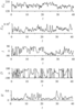
The first regime, see Figure 1, with the mesh grids $32^3$ corresponds to the slow rotation with ${\rm Re}\sim 20$.
The relative influence of rotation on hydrodynamics is measured by the Rossby number ${\rm Ro}$, which is equal to the ratio of the typical convective velocity to the daily rotation velocity. Rotation is important when ${\rm Ro}\ll 1$. In our case ${\rm Ro}= {\rm Re}\, {\rm E}\approx 0.6$.
It is useful to introduce mean kinetic $\displaystyle E_K={1\over 2 }\, \int V^2\, d{\cal V}$ and magnetic $\displaystyle E_M={1\over 2\, {\rm Ro} }\,\int B^2\, d{\cal V}$ energies over the spherical shell volume ${\cal V}$. As it follows from Figure 1, the time averaged ratio of these energies ${\cal R}=E_M/E_K\approx 3$, that is too small compared with that one in the Earth's core ${\cal R}_\oplus\sim 10^3$, see discussion in [Reshetnyak and Sokoloff, 2003].
Fluctuations of the magnetic and kinetic energies are anti-correlated, so that $E_K+E_M$ is constant. There is chaotic wobbling of the magnetic dipole at the middle latitudes. Only during time interval $t\in [22,\, 28]$ inclination $I$ of the magnetic field corresponds to the high latitudes. This regime is characterized by the frequent excursions of the field, when dipole intensity drops in three-five times and then recovers with the same sign. This regime satisfies to the criteria for the critical Rossby number ${\rm Ro}^c\sim 0.12$ introduced in [Christensen and Aubert, 2006], [Schrinner et al., 2010]. Accordingly to this estimate regimes with ${\rm Ro}<{\rm Ro}^c$ correspond to the geostrophic states with the non-reversing magnetic dipole located in the Taylor cylinder. Increase of ${\rm Ro}$ leads to the break of the geostrophic state accompanied with the chaotic reversals of the magnetic field. The magnetic dipole easily migrates from the Taylor cylinder to the outer region and back. Note, that correlation between the dipole intensity $H$ and inclination $I$ is absent. Moreover, evolution of $H$ does not correlate with evolution of the total magnetic energy in the liquid core $E_M$. The direction of the azimuthal drift of the dipole alternates in time, so that $\dot{D}$ changes its sign. This regime is quite different from that one in the Earth and corresponds to the low magnetic energy state with the magnetic dipole in the middle latitudes.
 |
| Figure 2 |
One of the ways to enlarge ${\cal R}$ is to increase the magnetic Reynolds number ${\rm R_m}$. It can be done in two ways: increasing velocities, either increasing the Roberts number $\rm q$ (decreasing magnetic diffusion). It is believed, that for the core the first scenario is realized ${\rm Re}\sim 10^8$, ${\rm q}=10^{-6}$ and ${\rm Ra}=10^{14}$ [Jones, 2010]. With change of ${\rm Ra}$ the following scalings is observed: ${\rm Ra}$ – $0.65:1$, ${\rm Re}$ – $1:1.5$, ${\rm R_m}$ – $1:9$, i.e. the slight increase of the heat source intensity leads to the significant increase of ${\cal R}\approx 70$, which is already closer to that one in the core. The price is increase of the already quite high Rossby number, which for the tested regime is ${\rm Ro}\approx 0.85$. In other words, increase of ${\rm Ra}$ enhances the spherical symmetry of the averaged in time physical fields, so that magnetic dipole location is even less connected to the geographic axis and dipole intensity does not correlate with the total magnetic energy of the core. The origin of such a weak connection can be understood from the analysis of the magnetic spectra. For this aim we consider the azimuthal $l$-spectra, derived from decomposition on the Schmidt semi-normalized harmonics $Y_l^m$, see Figure 2. The kinetic energy spectra has maximum at $l\sim 3$, whereas maximum of the magnetic energy $E_M$ spectra locates at the scale even smaller than $E_K$. So as ${\rm R_m}/{\rm Pe}={\rm q}\gg 1$, the small-scale generation of the magnetic field is quite intensive.
The other important characteristic of the geomagnetic field is the ratio of the dipole to the quadruple components ${\cal C}$. Using standard definition of the Mauersberger-Lowes spectrum [Langel, 1987]:
\begin{equation} \tag*{(4)}\label{4} R_l=(l+1)\left({R_\oplus\over r}\right)^{2l+4}\, \sum \limits_{m=0}^{l_{max}} \left( g_l^{m\, 2}+h_l^{m\, 2} \right), \end{equation}
where for the sources related to the liquid core $l_{max}=14$, and $g_l^m,\, h_l^m$ are the Gauss coefficients, the ratio is defined as $\displaystyle {\cal C}={R_1\over R_2}$. Then for the considered two regimes at the surface of the Earth, at $r=R_\oplus$, ${\cal C}=3.8$ and $2.8$, instead of the much larger estimates of $\displaystyle {\cal C}_\oplus=17.7$ for the modern geomagnetic field, see, e.g. IGRF-2010. For the liquid core surface $\displaystyle {\cal C}_\circ=1.3$ and $0.98$, and extrapolation of the observed geomagnetic field through the mantle ((4)) leads to $\displaystyle {\cal C}_\circ=\left({R_\oplus\over r_\circ}\right)^{-2} \cdot {\cal C}_\oplus \approx 1.7^{-2}\cdot 17.7 \approx 6.1$.
It is obvious, that to satisfy conditions ${\cal R}\gg 1$ and ${\rm Ro}\ll 1$ simultaneously at the large Ekman numbers is impossible and one needs to increase $\Omega$. This transition requires finer resolution and change of the grid to $64^3$.
 |
| Figure 3 |
The next regime with ${\rm Ro}=0.19$, see Figure 3, locates near the critical boundary ${\rm Ro}=0.12$.
\fitopen{1.073} Solution is characterized with a strong outbursts of the magnetic energies accompanied by the quite smooth evolution of the kinetic energy. At the pikes of $E_M$ the value of ${\cal R}\sim 20$ is quite high. At the time interval $t\in [5,\, 15]$ correlation of $E_M$ and magnetic dipole intensity $H$ is observed. The reversals are seldom. Mainly during the whole time interval dipole drifts in the western direction, $\dot D <0$. Increase of ${\rm Ra}$ in factor 1.5 causes enhance of $E_K$ in 2.3 times (so that ${\rm Ro}\sim 0.29$) and of the magnetic field energy in one order. Correlation between $E_M$, $I$ and $H$ with increase of ${\rm Ra}$ decreases substantially. Note, that simulations with the higher resolution reproduce the more typical for the geomagnetic observations behavior of the magnetic spectra at the core surface. For the both regimes $\displaystyle {\cal C}_\oplus\approx 4.1$ and $\displaystyle {\cal C}_\circ\approx 1.4$. As before, spectrum of the magnetic field slowly decays with increase of $l$. At $l=16$ there is the well-known extremum of the field related to the bottleneck effect, see for details [Canuto et al., 1988].
 |
| Figure 4 |
In conclusion we consider the model with the finer resolution $128^3$, with the Rossby number ${\rm Ro}=0.04$ and energies ratio ${\cal R}=50$, The observed force balance is the closest to that one in the Earth, see Figure 4.
 |
| Figure 5 |
There are three well-resolved reversals of the magnetic field. After the third reversal there is an excursion of the magnetic field at $t\approx 0.85$. All reversals appear during decrease of the magnetic energy $E_M$, which in its turn is correlated with the dipole field intensity $H$. The excursion is also appears when $H$ is decreased. Magnetic dipole rotates in the west direction, $\dot D<0$. As we have seen before, the slight increase of ${\rm Ra}$ leads to decrease of correlation between $E_M$, $H$, $I$ and change of the sign of $\dot D$. The $l$-spectra of the fields in Figure 5, decays slowly, as in the previous examples.
Contribution of the dipole component to $R_l$-spectrum is comparable to the previous cases as well: $\displaystyle {\cal C}_\oplus\approx 4$ and $3.2$ and $\displaystyle {\cal C}_\circ\approx 1.4$ and $1.1$, that is smaller than the desirable value in the core. \fitclose
Development of the 3D geodynamo models made possible to reconsider meaning of the paleomagnetic field observations and its significance for understanding of the processes in the liquid core of the Earth. In spite of the fact, that reversals of the geomagnetic field at the surface of the Earth relate to the substantial change of the total magnetic field, the corresponding variations of the mean quantities inside of the liquid core during the reversals have quite moderate amplitudes. Using the 3D dynamo model in the spherical shell with a various levels of geostrophy of the flow we demonstrated how change of the spectra of the kinetic and magnetic energies in the liquid core influence on interpretation of the paleomagnetic field observations and on the role of the reversals in the full dynamo problem. We show, that during the break of geostrophy in the liquid core contribution of the field at the small scales to the magnetic spectrum is comparable with the dipole component. As a result during the reversals of the field decrease of the dipole component is compensated with the slight increase of the spectrum at the high wavenumbers. This redistribution of the magnetic field does not produce significant changes in the hydrodynamics of the core.
Buchlin, E. (2011), Dynamo model with thermal convection and with the free-rotating inner core, Planet. Space Sci., 50, 1117–1122.
Canuto, C., M. Y. Hussini, A. Quarteroni, and T.A. Zang (1998), Spectral methods in Fluids Dynamics, Springer.
Christensen, U., P. Olson, and G. A. Glatzmaier (1999), Numerical modeling of the geodynamo: A systematic parameter study, Geophys. J. Int., 138, 393–409, doi:10.1046/j.1365-246X.1999.00886.x
Christensen, U., and J. Aubert (2006), Scaling properties of convection-driven dynamos in rotating spherical shells and application to planetary magnetic fields, Geophys. J. Int., 166, 97–114, doi:10.1111/j.1365-246X.2006.03009.x
Christensen, U., J. Aubert, and. G. Hulot (2010), Conditions for Earth-like geodynamo models, Earth Planet. Sci. Lett., 296, 487–496, doi:10.1016/j.epsl.2010.06.009
Frisch, U. (1995), Turbulence: The Legacy of A. N. Kolmogorov, Cambridge University Press.
Glatzmaier, G. A., and P. H. Roberts (1995), A three-dimension self-consistent computer simulation of a geomagnetic field reversal, Nature, 377, 203–209, doi:10.1038/377203a0
Gubbins, D. (2001), The Rayleigh number for convection in the Earth's core, Phys. Earth Planet. Int., 128, 3–12, doi:10.1016/S0031-9201(01)00273-4
Hollerbach, R., and C. A. Jones (1993), Influence of the Earth's inner core on reversals, Nature, 365, 541–546, doi: 10.1038/365541a0
Hejda, P., and M. Reshetnyak (2009), Effects of anisotropy in the geostrophic turbulence, Phys. Earth Planet. Int., 177, 152–160, doi:10.1016/j.pepi.2009.08.006
Jacobs, J. A. (1994), Reversals of the Earth's Magnetic Field, Cambridge University Press, doi:10.1017/CBO9780511524929
Jones, C. A. (2000), Convection-driven geodynamo models, Phil. Trans. R. Soc. London, A358, 873–897, doi:10.1098/rsta.2000.0565
Kuang, W., and J. Bloxham (1997), An Earth-like numerical dynamo model, Nature, 389, 371–374, doi:10.1038/38712
Kutzner, C., and U. R. Christensen (2002), From stable dipolar towards reversing numerical dynamos, Phys. Earth Planet. Int., 131, 29–45, doi:10.1016/S0031-9201(02)00016-X
Langel, R. A. (1987), The main field In Geomagnetism. Ed. J. A. Jacobs, 1, 249–512, Academic Press.
Reshetnyak, M., and D. Sokoloff (2003), Geomagnetic field intensity and suppression of helicity in the geodynamo, Izvestiya, Physics of the Solid Earth, 39, 9, 774–777.
Reshetnyak, M., and P. Hejda (2003), Direct and inverse cascades in the geodynamo, Nonlin. Proc. Geophys, 15, 873–880, doi:10.5194/npg-15-873-2008
Roberts, P., and G. Glatzmaier (2000), A test of the frozen-flux approximation using a new geodynamo model, Phil. Trans. R. Soc. Lond., A358, 1109–1121, doi:10.1098/rsta.2000.0576
Schrinner, M., D. Schmitt, R. Cameron, and P. Hoyng (2010), Saturation and time dependence of geodynamo models, Geophys. J. Int., 182, 675–681, doi:10.1111/j.1365-246X.2010.04650.x
Schubert, G. (2007), Core dynamics In Treatise on Geophysics. Ed. P. Olson 8 Elsevier.
Simitev, R. (2004), Convection and magnetic field generation in rotating spherical fluid shells, Ph.D. Thesis. University of Bayreuth.
Wicht, J. (2002), Inner-core conductivity in numerical dynamo simulations, Phys. Earth Planet. Int., 132, 281–302, doi:10.1016/S0031-9201(02)00078-X
Received 23 November 2012; accepted 13 March 2013; published 17 March 2013.

Citation: Reshetnyak M. Yu. (2013), Geostrophic balance and reversals of the geomagnetic field, Russ. J. Earth Sci., 13, ES1001, doi:10.2205/2013ES000526.
Copyright 2013 by the Geophysical Center RAS.