Behavior of the galactic cosmic ray intensity at solar minima periods

M. S. Kalinin and M. B. Krainev

P. N. Lebedev Physical Institute, Moscow, Russia

Contents

Abstract

1. Introduction

The data obtained by a network of spacecraft (IMP 8, Pioneer 10, and Voyager 2) during more than 2 decades and covering large spatial scales (up to r = 65 AU) allow comparative analysis of the GCR intensity behavior during two successive 11-yr solar cycles. In spite of a limited amount of data, this analysis [Webber and Lockwood, 1997] has revealed a rather unexpected intensity behavior in the distant heliosphere. If we consider only successive solar minima - the GCR intensity measured by IMP 8 ( r = 1 AU) in 1996 was approximately equal to that in 1976 - an unexpected very weak increase in the GCR intensity with radial distance is revealed in the distant heliosphere ( r 40 AU) in 1995-1996 as compared with 1987. For the 130-230 MeV proton channel, the ratio between intensities in 1996 and 1987 was J₉₆/J₈₇ 1.23 at the Earth's orbit, 0.44 at r 42 AU, and as low as 0.29 at r 64 AU.

These data, supplemented by Ulysses data on global latitudinal GCR gradients [Heber et al., 1996] and spectra measured by IMP 8 at the Earth's orbit, have been described by numerical solutions of the transport equation with standard boundary conditions [Potgieter, 1997]. It has been shown that in order to satisfactorily describe the spatial GCR distribution in the heliosphere at two successive intensity maxima (solar minima) periods, the main parameter of the model - radial diffusion coefficient - should be taken to be 5-6 times greater for the intensity maximum in 1987 (when the radial projection of the interplanetary magnetic field in the Northern Hemisphere was negative, A = -1 ) than for the intensity maximum in 1996 (when the projection was positive, A = 1 ). Another characteristic of the spatial distribution - latitudinal intensity gradients at 40-60 AU - proved to be too small for the period with A = -1 in this case.

The goal of this work was to show, based on numerical solution of the transport equation for protons, that experimental data on the radial intensity behavior can be satisfactorily described if we introduce additional modulation beyond the outer heliosphere boundary due to the modulating action of the electrostatic potential that changes its sign at the TSMF polarity reversal.

2. Description of the Model

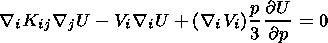
The spatial distribution of proton intensity was calculated by numerically solving the two-dimensional (with respect to spatial variables r (radial distance) and q (polar angle)) axisymmetric stationary diffusion equation including drift [Toptygin, 1983]

(1)

where U is the particle density in the phase space (  r,p) related to the intensity J as J = p²U; K_ij is the total diffusion tensor (DT) whose nonsymmetric part describing drifts corresponds to coefficients K_T K_Tf(q,a) for the tilt angle of the current sheet of a = 5^o modified according to Potgieter and Moraal [1985] and Jokipii and Kota [1989]; and V_i is the solar wind (SW) velocity having only radial component depending on both spatial coordinates. The actual dependence of the SW velocity on coordinates was qualitatively consistent with the Ulysses data and was approximated as

(2)

where r₀ is the photosphere radius. At q< 60^o, the SW velocity was latitude-independent and corresponded to the solution of (2) for q = 60^o.

The symmetric part of the DT describing diffusion was taken to be fully anisotropic; and the components normal to the magnetic field were assumed to be proportional to the field-aligned component K _r = a₁K, K _q = a₂K. Fixed coefficients a₁ and a₂ were chosen so as to fit the radial intensity behavior and to ensure the ratio between the intensities at the pole and helioequator for radial distances r 1 AU limited by 1.4-1.5 [Heber et al., 1996]. The field-aligned diffusion coefficient is given by

(3)

Here, the dimensional coefficient K₀ measured in terms of 6 10²⁰ cm² s^-1 was adjusted in calculations; b = n /c, where n is the particle velocity and c is the speed of light; and function f₁(R), where R is rigidity, was chosen so as to fit experimental data. In practice, a simple dependence

(4)

was used.

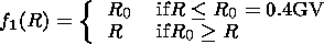
The antisymmetric coefficient K_T describing drift was taken in the standard form K_T = K₀^(a) f(q, a) b R/3B, where B is the value of the interplanetary magnetic field (IMF); and coefficient K₀^(a), typically equal to unity, was varied to control the effect of drift. Function f₂(r) = 1 +rⁿ, where r is expressed in AU.

Equation (1) was solved with the standard initial condition U( r,p_m) = U_H(p_m), where U_H(p) is the unmodulated particle density in the Galaxy, p_m = 100 GeV s^-1, and conditions at the outer boundary r = r_M of the modulation region are U(r_M, q, p) =U_H(p).

The effect of external modulation beyond the modulation region was provided by the modulating action of the electrostatic potential (EP), which was described by the expressions obtained earlier by Kalinin and Krainev [1992, 1997] (see also Krainev [1979] and Jokipii and Levy [1979]), but shifted by the value a which was chosen so as to fit experimental data

(5)

where A = 1 indicates the TSMF polarity, r_s is the radius of the magnetic field source surface, w is the angular speed of rotation of the Sun, B_s is the radial component of the magnetic field at the source surface, and function f(q) describes the latitudinal dependence according to Kalinin and Krainev [1992]. In calculations, coefficient (Br₀²w/c) equal to 0.25 GV, typical of the heliosphere was used. The particle density was recalculated for the outer boundary of the modulation region by using the relation U(r_M, q, p) = U_H(p + Dp), where r_M = 100 AU is the modulation region radius (Liouville theorem). In this expression, p and p' = p + Dp are related by the energy integral

(6)

Here, q is the particle charge.

As a result, a radial intensity profile of the 200-MeV protons at the helioequator was obtained and then compared with the data of the 130-230 MeV proton channel at the spacecraft obtained by Webber and Lockwood [1997].

3. Calculations in Terms of Standard GCR Modulation Model

Figure 1

Procedure of calculations was as follows: at first, parameters K₀, a₁, a₂, and K₀^(a) were adjusted to fit the radial intensity behavior at A = 1 (in 1996) under standard boundary conditions. Throughout this section, the value n = 1 in the functional dependence of the diffusion coefficient on the radial distance is used. Because of low intensities in the distant heliosphere, it is impossible to describe satisfactorily the radial intensity behavior for the full drift coefficient K₀^(a) = 1. In this case, a too high-intensity in the distant heliosphere results. At abnormally low diffusion coefficients, at A = 1, the contribution of the drift mechanism is able to provide a sufficient intensity level. However, in this case too-large latitudinal gradients near the Earth's orbit, which are approximately three times as large as those derived from the Ulysses data, are obtained. Therefore, it is necessary to considerably reduce the contribution of the drift mechanism and increase the diffusion coefficients to the values providing actual latitudinal and radial gradients. Fitting results for K₀^(a) = 0.5 are shown in Figure 1a. Hereinafter, the experimental points corresponding to the intensity maximum in 1996 are shown by crosses, and the data for 1987 are shown by diamonds. Note that the point at A = -1 and r = 64  AU does not indicate the actual intensity; it is the result of extrapolation of the intensity at r= 42 AU. Solid lines show the calculated radial intensity behavior for A = 1. Figure 1b presents calculated spectra in comparison with the spectra obtained by IMP 8 for the same time periods. UMS denotes the unmodulated spectrum at the modulation region boundary.

It is clear from the magnitudes of the parameters given in the caption to Figure 1 that even in the case of a two-fold decrease in drift effects, coefficient K _r, responsible for radial gradients in the distant heliosphere, must be chosen low enough to provide the required large intensity drop within the interval of distances 20 AU from the outer boundary of the modulation region.

Figure 2

On the contrary, in the middle and also in the near heliosphere, where radial gradients, according to Webber and Lockwood [1997], are small, coefficient K should be sufficiently high to provide these small radial gradients. The relevant latitudinal dependence of intensity for A = 1 and r = 1 AU is shown in Figure 2. To provide the required latitudinal gradient, the coefficient K _q should exceed K _r approximately by a factor of 10.

Figure 3

Figure 1 demonstrates that with the values of parameters fitting the intensity at A = 1, the intensity at A = -1 proves to be strongly suppressed, especially in the near heliosphere, and does not fit the experiment. A reasonable result for A = -1 can be obtained only by increasing the coefficient a₁ (that is, K _r) by a factor of 5-6. In this case, realistic latitudinal gradients for radial distances of ~1 AU result. Calculations and also initial parameters are shown in Figure 3. It is evident that in this case, the situation at A = 1 is not described.

Figure 4

Figure 4a demonstrates the radial intensity behavior for A = -1 at different heliolatitudes (approximately in 10^o intervals, the upper line at r 20 AU corresponds to the intensity at the helioequator). It is obvious that the negative latitudinal gradient changes the sign at distances 20 AU. However, as shown in the right-hand panel (b) presenting latitudinal intensity dependence for A = -1 at radial distance 64 AU, this maximum latitudinal gradient does not exceed 1%/AU. It is by a factor of 2-3 lower than the experimental estimates given by Webber and Lockwood [1997] for r = 42 AU and extrapolated to r = 64 AU.

The major conclusion inferred from the above consideration is that the transport equation is not able to describe the experimental spatial GCR distribution within the heliosphere at successive solar minima periods in terms of the standard approach involving the same set of kinetic coefficients. To adequately describe measurements, at least the diffusion coefficients responsible for the radial distribution of the GCR intensities must considerably differ in these sets (by a factor of 5-6).

Thus, the obtained results confirm the conclusions made by Potgieter [1997], who considered an analogous problem in terms of another model dependence of the diffusion coefficients on the rigidity. Note also that our results are not the consequence of the diffusion coefficient dependence on the radial distance in the form K (1+r) that we have chosen. For instance, the K 1/B dependence (where B is the IMF value) often used gives the same qualitative picture. The difference is in insignificant changes in the transport equation parameters.

4. Effect of "External" GCR Modulation by the Electrostatic Potential of the Heliosphere

The results given in the previous section suggest that other modulating factors can exist. By considering them, it is possible to avoid inconsistencies arising in description of the measured spatial GCR distribution. It is quite natural that these factors must be associated with the Sun - the only cause and source of modulation - and, in addition, they must exhibit a "correct" dependence on the sign of the 22-yr solar cycle phase (that is, on the sign of A ) and on heliolatitude. In a correct dependence, the effects of these factors fit the experimentally observed GCR behavior.

If we extend the radial intensity dependence to the outer heliosphere boundary using the same gradients as in the distant heliosphere, it becomes evident that two successive solar minima can have different intensity levels at the outer heliosphere boundary. In this case, the ratio between unmodulated intensities for the energy interval considered must be 3-4. However, the attempt to describe the radial intensity behavior at two successive solar minima by varying only the value of the intensity spectrum at the modulation region boundary, without changing its shape (that is, with unvaried energy dependence), and by using the same set of transport equation coefficients for different signs of A is not justified, on the one hand, and does not give the desired result, on the other hand.

Kalinin and Krainev [1992, 1997] derived the expression for the heliospheric electrostatic potential (EP) averaged over the azimuthal variable relative to infinity on the basis of the Parker spiral IMF structure and high electric conductivity of the SW plasma. Since the EP induced in this heliosphere model is completely included in the transport equation, which is solved for the inner regions of the heliosphere, the action of such induction field beyond the heliosphere can be reduced, in the first approximation, to the effect of its EP on the intensity spectrum at the heliosphere boundary. In this case, the dependence of EP on global sign-defining multiplier A describing polarity of the 11-yr cycle and on latitude provides the necessary and correct dependence on it of the modulating effect beyond the heliosphere. The EP value necessary to provide the required modulation level at the modulation region boundary for different A is determined by the intensity difference in the distant heliosphere. It depends also on how completely physical mechanisms affecting the true unmodulated intensity spectrum at large distances beyond the heliosphere are taken into account. If we ignore energy losses of particles during their travel to the outer heliosphere boundary from the local interstellar medium and assume the efficient action of nondissipative scattering, the particle density along their trajectories in the phase space must be preserved, according to the Liouville theorem. If, in determining the phase trajectories, we restrict ourselves to the EP effect and ignore the IMF influence, all trajectories will belong to the constant-energy surfaces with uniform filling. In this case, the spectrum at the modulation region boundary can be found from the expression: U( r_M, p) = U_H(p') (see the expression in the above discussion). Note that this approach can be regarded only as the first approximation to the actual picture, but it is useful owing to its simplicity [Jokipii and Levy, 1979].

The qualitative picture of the modulating EP effect beyond the heliosphere in terms of the approach described above is sufficiently clear and follows from (6). It is not reduced to a mere change in the spectral amplitude at the heliosphere boundary. For the period with A = -1, the EP effect at low latitudes leads to a considerable shift of the initial unmodulated intensity spectrum toward higher kinetic energies (that is, the spectrum goes higher and simultaneously is cut from the left).

Figure 5

The effect of this modulation on the intensity spectrum in the low-latitude region at A = 1 is much weaker. In this case, the spectrum shifts to the left, that is, it becomes lower than the initial unmodulated spectrum. However, in the high-latitude region, from which positively charged particles are transported by drift to low latitudes at A=1, the picture is inverse. The intensity spectra recalculated to the modulation region boundary for EP resulting from the parameters typical of the heliosphere are shown in Figure 5 for different  A.

Thus, the intensity spectrum at the heliosphere boundary for any above-threshold energy determined by the EP amplitude (~125 MeV) at A = 1 is lower in near-equatorial regions and higher in the polar regions as compared with that at A = -1, thereby providing the necessary sign of the effect. In addition, this picture of the influence on the unmodulated intensity spectrum should lead to increasing latitudinal gradient in the distant heliosphere, thus providing a better fit to measurements.

Figure 6

In calculations, the expression for EP obtained by Kalinin and Krainev [1992] but shifted by a constant value a (in units of amplitude value Br₀²w/c) chosen so as to fit the radial dependence was used. The latitudinal dependence of EP for both polarities of the 11-yr half-period of the solar cycle and a = 0 is shown in Figure 6.

Figure 7

To obtain the necessary value of EP, parameter a was varied with a step of 0.1 (in units Br₀²w/c) within the interval 0-0.5. This corresponded to changes in j_G from the values typical of the heliosphere to the values shifted upward by Br₀²w/2c 0.125 GeV, the latitudinal dependence remaining the same. The qualitative picture of the EP effect on the radial intensity behavior for different A and relevant transport equation coefficients (given under Figures 2 and 3) providing adequate description of the radial behavior without the EP effect is presented in Figure 7. The lower curve in panel (a) and the upper curve in panel (b) correspond to a = 0.5. Figure 7 demonstrates a higher sensitivity of intensity to the EP value in the distant heliosphere at A = -1. The intensity at distances 20 AU from the boundary drops more than by an order of magnitude. This is associated with a characteristic peak-like shape of the intensity spectrum in the region of energies approximately equal to the amplitude of j_G at A = -1. With this A, the EP effect on the intensity for a = 0 (the lower curve in panel (b)) is insignificant for radial distances 1-64 AU. On the contrary, at A= 1, the effect of the potential is more pronounced in the middle and near heliosphere because at positive A, the mechanism of particle drift from near-polar regions of the heliosphere toward the equator is efficient.

Figure 8

Proceeding from the general qualitative picture of the EP effect on radial intensity distribution described above, diffusion coefficients were taken to be intermediate between the coefficients fitting spatial distribution at A = 1 and A = -1 in the absence of the EP effect and to be equal to each other for A of both signs. The radial intensity behavior for a = 0.5 shown in Figure 8 demonstrates that EP corresponding to this a is able to provide a necessary intensity difference in the distant heliosphere. However, the intensities for radial distances r 40 AU go higher than the experimental points. An intensity decrease can be achieved only by limiting the linear growth of the diffusion coefficient with 1 +r by the values corresponding to some radial distance r_P. A reasonable result given in Figure 8 (panel (b)) can be obtained for r_P = 50 AU. Figure 8 shows that the radial intensity behavior at A= -1 is more sensitive to the EP value than at A = 1. In addition, the intensity at A = -1 in the distant heliosphere remains somewhat higher than the experimental values. Since the point at r = 64 AU was obtained by extrapolating the intensity at 42 AU (see above), and measurements for r 64 AU are not available, this difference cannot be considered significant.

Figure 9

The behavior of the EP-modulated intensity at the modulation region boundary near the helioequator at A = -1 leading, for the energies considered, to overestimated intensities in the distant heliosphere is determined to a large extent by the method of recalculation of unmodulated spectra to the modulation region boundary that we used. This method does not take into account dissipative processes (adiabatic losses). Their effect on the spectra at the modulation region boundary can be most rigorously taken into account only by solving the full transport equation. At present, this is hardly possible because there is no model of spatially distributed EP. In the first approximation, the action of such "smoothing" effects can be achieved by increasing the modulation region radius. In a larger modulation region all methodical effects are "suppressed" within the intermediate region 20 AU near the outer boundary. The calculations and the values of coefficients used are shown in Figure 9a. Panel b of Figure 9 presents the calculated spectra for r = 1 AU.

5. Conclusions

The obtained results show that

1. It is impossible to fit the measurements of spatial GCR distribution in the heliosphere at successive solar minima in terms of the standard approach to the solution of the transport equation involving the use of the same set of diffusion coefficients. There is a question: whether the difference in transport equation parameters corresponds to the difference in actual physical conditions of the GCR particle propagation in the heliosphere at successive solar minima periods is distinguished, according to modern ideas, only by the TSMF sign. The question still remains unresolved.

2. Since the required difference in diffusion coefficients is associated with a low intensity level in the distant heliosphere at the solar minimum when the TSMF sign was positive and the drift mechanism had to be effective, the question about the actual contribution of drifts into modulation arises. The contribution of drifts derived from the standard first-order orbit theory is likely to be overestimated, and the fit to measurements can be achieved only by assuming the contribution of this mechanism to be half its standard value. Since a much lower radial diffusion coefficient in the distant heliosphere is also required to fit measurements during this period, this result can be interpreted as the effect of diffusion on the drift efficiency (a low diffusion coefficient corresponding to intense scattering leads to a weaker drift mechanism).

3. One of the ways to avoid inconsistencies accompanying the standard approach is to assume that the radius of the Sun's action on charged GCR particles extends beyond the boundaries of the modulation region, which is typically thought of as heliosphere sizes. A direct physical mechanism in this case is the EP effect on the GCR intensity spectrum beyond the modulation region. According to the results given in section 3, the EP having the amplitude of 250-300 MV and depending on the TSMF sign is needed to fit measurements. This potential differs from the EP typically associated with the heliosphere by a shift by a constant value, Br₀²w/2c 125 MV; the latitudinal dependence remains unvaried. This EP value can be associated with the positively charged heliosphere when the total charge within any radius is not zero. This possibility cannot be excluded, though there are no arguments in favor of this hypothesis as well. Another possible way to increase the EP amplitude can be taken into account: the latitudinal dependence of the magnetic field at the source surface, which is usually neglected for simplicity [Krainev, 1981]. Consideration of both assumptions is beyond the scope of this paper. In conclusion, a conceptually similar approach, but in terms of a more realistic model, was successfully employed by Jokipii and Kota [1997] to describe the radial behavior of the anomalous CR component.

References

Heber, B., et al., Spatial variation of > 40 MeV/n nuclei fluxes observed during the Ulysses rapid latitude scan, Astron. Astrophys., 316, 538, 1996.

Jokipii, J. R., and J. Kota, The polar heliospheric magnetic field, Geophys. Res. Lett., 16 (1), 1, 1989.

Jokipii, J. R., and J. Kota, The energy spectrum of anomalous cosmic rays, in Proceedings of the 25th International Cosmic Ray Conference, vol. 2, pp. 229-232, Durban, 1997.

Jokipii, J. R., and E. H. Levy, Electric field effects on galactic cosmic rays at the heliospheric boundary, in Proceedings of the 16th International Cosmic Ray Conference, vol. 3, pp. 52-56, Kyoto, Japan, 1979.

Kalinin, M. S., and M. B. Krainev, The electromagnetic heliospheric field and galactic cosmic rays during the periods of low solar activity, in Mathematical Models of the Near Space, Proceedings of the 2nd National Meeting in Memory of V. P. Shabanskiy (in Russian), Moscow University, Moscow, 1992.

Kalinin, M. S., and M. B. Krainev, The electric field beyond the termination shock and some possible GCR and ACR effects, Adv. Space Res., 19 (6), 969, 1997.

Krainev, M. B., The solar corona expansion geometry and cosmic ray effects, IV, On the cosmic ray energy change due to the electric field, in Proceedings of the 16th International Cosmic Ray Conference, vol. 3, pp. 236-241, Kyoto, Japan, 1979.

Krainev, M. B., The electromagnetic field in and outside the solar wind cavity and the galactic cosmic rays, in Proceedings of the 17th International Cosmic Ray Conference, vol. 3, p. 357, Paris, 1981.

Potgieter, M. S., Applications of enhanced perpendicular diffusion in the heliospheric modulation of cosmic rays, in Proceedings of the 25th International Cosmic Ray Conference, vol. 2, pp. 1-4, 1997.

Potgieter, M. S., and H. Moraal, A drift model for the modulation of galactic cosmic rays, Astrophys. J., 294 (2), 425, 1985.

Toptygin, I. N., Cosmic Rays in the Interplanetary Magnetic Fields (in Russian), Nauka, Moscow, 1983.

Webber, W. R., and J. A. Lockwood, Intensities of anomalous and galactic cosmic rays in the outer heliosphere near the heliospheric equator in 1987 and during the period from 1994 to 1996, J. Geophys. Res., 102, 9773, 1997.