Quantitative explanation of satellite ionograms taken within the F2-layer maximum

N. P. Danilkin and N. G. Kotonaeva

Institute of Applied Geophysics, Moscow, Russia

Contents

Abstract

1. Introduction

Figure 1

As a result of the satellite radiosounding from altitudes below the F -region maximum ionograms of a new type have been recorded [Danilkin, 2001]. These ionograms have new extra features which (as far as the authors know) have never been detected in any topside sounding experiment. These new features encouraged us to provide more complete description of the properties of the medium studied by the radiosounding method. A typical feature of the above mentioned ionograms is the continuation of the trace reflected from the surface. Figure 1 illustrates this fact, showing two ionograms recorded in the ionospheric radiosounding experiment on board the Mir space station.

In the first publication Danilkin [[2001] called quite conventionally the extra trace the "lower trace," the name emphasizing its position on the ionogram at the "virtual distance" axis. The ionogram in Figure 1 (left) shows the left end of the lower trace at the critical frequency of the F2 -layer ordinary component ( f_oF2 ). Such situation was predicted by Danilkin and Vaisman [1977] on the basis of numerical simulation of the ionosonde behavior on board the Mir station orbiting below the main electron concentration maximum in the ionosphere ( h_mF2 ). The first explanation of this trace was that it is a result of consequent reflections from the layers above the satellite location followed or preceded by the reflection from the surface. However, explanation of the lower traces became more difficult when it became known that in the majority of cases the lower trace is not limited by the f_oF2 frequency but goes much higher, as can be seen in Figure 1 (right).

Danilkin [[2001] assumed that possible cause of the occurrence of the lower trace with the right-hand end near the uppermost frequency of the ionosonde emission may be the presence of significant horizontal gradients of the electron concentration in the radiosounding zone and, as a result, the existence of rays returning to the satellite. The above described qualitative explanation of the observed effect has caused many questions. First of all, what horizontal gradients should exist to make possible a realization of the above mentioned oblique rays. No experimental data in which such trajectories have been recorded or calculated were known to the authors. Therefore existence at many frequencies of returning trajectories with very peculiar group delays detected in our experiments needs to be proved by numerical simulation methods.

In this paper the above mentioned hypothesis on horizontal gradients being a cause of the extra, so-called lower, traces in the ionograms recorded at the Mir station is checked quantitatively. The method of N(h) -profile calculations for a satellite situated below the F2 -layer maximum is a fragment of the general case studied in this work and described in section 3.

2. Method of Trajectory Drawing

To check quantitatively the existence of returning trajectories in the conditions of considerably irregular ionosphere, the iteration scheme first described by Lawrence and Posakony [1961] has been chosen. The scheme of ray calculations in an isotropic ionosphere was used to clarify principal questions. For more accurate calculations and in the conditions when the frequency close to the gyrofrequency were considered, the relations typical for the anisotropic ionosphere and described by Lawrence and Posakony [1961] were used. To avoid introduction of cumbersome formulae typical for the refraction index description in anisotropic medium, in this paper we describe only the first scheme.

While drawing trajectories, we used three key assumptions: (1) the layering of the ionosphere (the space is divided into layers of the same thickness in such a way that all the parameters within a layer are considered the same and between the layers vary so slightly that one can neglect the reflected wave at the interface); (2) the isotropic ionosphere; (3) as a result of the isotropy, a plain curve trajectory with its wave normals always being parallel to the incidence plane and satisfying the refraction law.

The trajectory calculation actually consists of two stages: (1) calculation of the vertical or oblique trajectory from the satellite to the surface; and (2) calculation of the return trajectory after reflection from the surface and aimed at the satellite with necessary accuracy. We calculated the N(h) profile needed for drawing the trajectory using known methods. Initially, it was calculated using the Danilkin and Mal'tseva [1977] method directly from the ionogram between the satellite real height and the height of the F2 -layer maximum using the o and x components reflected from the ionosphere (see Figure 1).

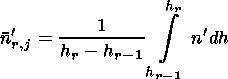
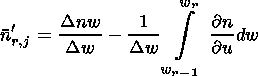
The N(h) -profile calculation was performed in the following way. First, a series of frequencies f_r with corresponding true h_r and virtual reflection heights h'_r is taken. They are related by

(1)

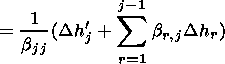
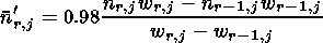
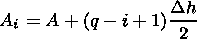
where n' is the group refraction index and n'_r,j is its mean value for the f_j frequency in the layer between h_r-1 and h_r.

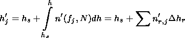
Thus the virtual reflection height h' for a radio wave with a frequency f_j and vertical incidence on the ionosphere is

(2)

where h_s is the satellite altitude and h is the height above the Earth surface.

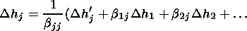
Designating h_s = h'_s, n'_r,j-1 - n'_r,j = b_r,j (r j), n'_jj = b_jj, we obtain recursive formulae for the excess of the true height:

(3)

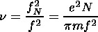
The coefficients n'_r,j are calculated for a particular position of the satellite depending on the gyrofrequency value f_h and magnetic inclination q. With the modern high computation rate this is convenient even for calculations at different points of the globe.

To calculate the n'_r,j coefficients, an assumption is made that h is a linear function of w=1/n ^1/2 at the unit segment [h_r-1; h_r], where

and, consequently, w = f/f_N. Using this assumption to determine n'_r,j, we have

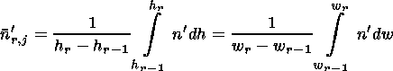The refractive index is described by the standard formula and is a function of two variables u and n, where u = f_h/f:

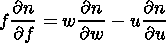(4)

where n is the phase refraction index.

For the ordinary component, the second term in equation (4) is small (not more than 2% of the first term) and constant; thus the group refraction index for a frequency f_j in the h_r-1 - h_r layer is

Using the relations presented above to calculate the coefficients of system (3), we are able to find the excess of the true height and, respectively, the entire N(h) profile. If there is a need to calculate the N(h) profile using the extraordinary component, the corresponding relations for it are calculated in the same way.

The N(h) profile below the satellite height is determined on the basis of the foundations of the vertical transionosphere sounding [Danilkin, 1994] using the ordinary traces of the signals reflected from the surface. The profile from the ionospheric bottom up to the F -region maximum height obtained in the way described above was used in the above mentioned first stage of the calculation of the trajectory from the satellite to the surface. The back-scattered trajectories were found by the consequent approximation method. The first "oblique" trajectory was vertical and used (after the comparison of the calculated virtual distance with the experimental virtual depth of the reflection from the surface determined from the ionogram) to control and specify the N(h) profile. The direction of the second ray was chosen at some angle to the vertical, and its frequency was slightly higher than the plasma frequency of the ionosphere at the satellite height. In the ionosphere without horizontal gradients, such a ray after reflection from the surface would go into the ionosphere far from the satellite. In order for this trajectory to return to the satellite (as is observed in the experiment), after reflection from the surface, the ray should propagate in the ionosphere with parameters significantly different from the parameters of the ionosphere in which the ray propagated to the surface. In other words, the ray should be close enough to an "irregularity" and its trajectory should be influenced by horizontal gradients.

Parameters of such an ionosphere are fitted by one of several ways described below until the ray hits the satellite with a given accuracy. We then achieve a coincidence of the experimental and calculated virtual distances determining the deviation angle from the vertical and each time drawing the trajectories returning to the satellite and integrating along them the group delays.

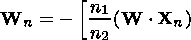
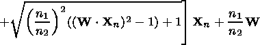
To calculate the first (vertical) trajectory, the aim point was chosen at the surface under the satellite ( X ). In this case the coordinates of the first wave normal vector are

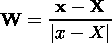where x is the satellite coordinate. The coordinates of the radial vector X_n of the points to which the ray comes moving along the W vector up to an interception with the next layer are calculated by

(5)

where

is the length of the ray trajectory within one layer.

Crossing the interlayer boundary, the ray changes its direction according to the refraction law, still staying in the plane of the previous wave normal and normal to the surface, the latter in the case of a layered atmosphere being directed along the radius vector of a trajectory point. Therefore the coordinates of the new directing vector are defined as

(6)

Sequentially calculating the coordinates of crossing of every ionospheric layer and using formula (6), we obtain the ray propagation trajectory up to the exit from the ionosphere, where n= 1 and the directing vector W does not change and is taken to be equal to the wave normal vector in the last layer. Then the coordinates of the point of the radius vector interception with the surface are calculated by

The length of the ray trajectory within the ionosphere is given by

To calculate the wave normal directing vector W_E for from the surface, we assume an equality of the incidence and refection angles, so

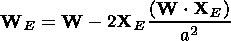(7)

Then the virtual distance h' for the motion along the trajectory is calculated. For the vertical incidence case this calculation is compared with the real distance derived from the ionogram and thus the correctness of the initial N(h) profile is checked. Since in the model in question the ray trajectory is piecewise, the following formula is true:

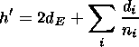(8)

where d_i is the trajectory length passed by the ray within the i th layer. The value of h' includes the virtual distances during the ray propagation from the satellite to the surface and the distances from the point of crossing the ionospheric lower boundary to the surface and back up to the ionosphere.

3. Introduction of Horizontal Irregularity

The simulations performed to explain ionograms of the type shown in Figure 1 have shown that all features of these ionograms may be explained if one assumes a reflection of the sounding ray from the surface and its consequent returning to the satellite as a result of its refraction at a strong ionospheric irregularity. Also, a reflection from the vertical (or oblique) walls of the types described earlier by Danilkin [[2001] is also possible. However, it would have required a stronger structure, and we did not included it in our calculations. Principally, it changes nothing except the calculation method itself. We failed to find any new explanation of all the details in new ionograms.

To draw trajectories "returning to the satellite after the surface reflection" (below we call them simply "returning trajectories"), one has to introduce an ionospheric irregularity. A simple consideration shows that an irregularity within which the electron concentrations in various layers or plasma frequencies exceed corresponding values outside the irregularity should turn the ray in the direction of the satellite. Such irregularities are usually called "positive," contrary to "negative" ones where the plasma frequencies are, respectively, lower than the background frequencies. Various methods to introduce ionospheric irregularities into radio circuit calculations are available. We have used the following two schemes, each of them making it possible not only to find returning trajectories but to get agreement with the virtual distances measured in the experiment.

In the first, more simple for realization, scheme, it is assumed that the normal vector to the surface after the reflection is directed not to the Earth's center but to some other point in the trajectory plane. Changing the position of this point, we obtain some sort of an inclination of isolines of the same electron concentration. The value of this inclination characterizes the degree of irregularity contrast. This method is very convenient for a geophysical analysis of irregularity occurrence in the global ionosphere, since it makes it possible to introduce the real coordinates of both the satellite position and the irregularity which has led to appearance of the "lower rays" in question. Difficulties of a description of the irregular ionosphere (which is passed through by the returning ray) in the vicinity of the satellite is a defect of this scheme.

To take into account irregularities, the second scheme assumes that the irregularity is introduced by a special function which is superposed on the undisturbed state of the ionosphere. A mathematical model of such ionosphere is a set of functions different from spherical ones. Plain layers are smoothly transformed into layers limited by Gauss-type curves. The refraction index within each layer is constant and corresponds to the index obtained from the ionogram.

Analytical expression for these curves is

where q is the layer number counted from the bottom of the ionosphere; (y_b, z_b) are the coordinates of the irregularity center in the Cartesian coordinate system, chosen in the following way. The center of the system coincides with the Earth center, the z axis goes though the satellite, and the satellite moves within the zy plane.

A_i and D_i are parameters of the curves calculated by

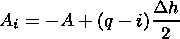for the layers located below the irregularity center and

for the layers located above the irregularity center, the A_i coefficients for symmetric layers being equal by the magnitude and opposite by sign. Then D_i = D |q -i|, the D_i coefficients for symmetric layers being the same; A and D are the irregularity parameters fitted as a result of the numerical simulation.

Within the irregularity, elliptical layers with the ellipse center located in the center of the irregularity are modeled, the semiaxes calculated by

where j is the number of the elliptical layer and T is the irregularity parameter.

The refraction index n_j within each layer with number j is also constant and determined from

where j=0 is the number of the last nonelliptical layer and j = 1, 2, , l are the numbers of the elliptical layers.

The T and k parameters as well as the number of elliptical layers l are fitted in the process of the numerical simulation. A sequent numbering is given to all layers. According to this numbering for every point of the space, there is a corresponding number of the layer in which the point is located.

Introducing the above described model, we determine for every point (y₀, z₀) two parameters: the refraction index n corresponding to the number of the layer the point is located in and the normal vector to the surface l_n located in the yz plane. The coordinates of this vector are calculated by

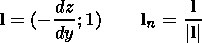Here dz/dy is a derivative (calculated for the y₀ point) of the function of the lower boundary of the layer in which the point (y₀, z₀) is located.

While propagating from the satellite to the surface, the ray is at significant distance from the irregularity center, so its influence on the signal trajectory is small. Because of that, calculating the trajectory of the ray propagating "downward," the mathematical model of a spherically layered ionosphere described in the previous section is used.

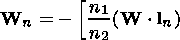
For the propagation after the reflection from the surface and crossing the bottom boundary of the ionosphere, the trajectory in the points with the radius vector I (y_i0, z_i0) along the directing vector W is calculated in the following way: (1) the distance step d propagated by the ray in one direction is taken (for example, 5 km); (2) using the formula X_n = I + d W, the coordinates of the radius vector X_n of the new point of the trajectory are determined; (3) the number of the layer in which this newly obtained point is located and corresponding refraction index and normal vector to the surface l _n are determined; (4) using the refraction law, the coordinates of a new wave normal W_n are calculated by the formulae similar to equations (6) and (7):

if a refraction occurs and the angle between the W and l _n vectors is obtuse or

if a refraction occurs and the angle between the W and l _n vectors is acute; W_n = W - 2 l_n ( W l_n), if refraction is impossible and a reflection of the ray occurs; and (5) using the formula X_n = X + d W_n, where X is the radial vector of the previous point, the coordinates of the radial vector of a new point of the trajectory are calculated, and so forth.

To calculate the virtual distance during the motion along the trajectory, a formula similar to (8):

is used, where h'₁ is the virtual distance from the satellite to the surface calculated with formula (5), K is the number of the calculation steps, and n_k is the refraction index in the layer where the point is located during the k th step.

4. Results

Figure 2

Figure 2 illustrates a calculation of the ionospheric N(h) profile and returning trajectories for the ionogram shown in the right-hand ionogram in Figure 2.

A ionogram with very characteristic lower trace in the range of high frequencies has been deliberately chosen. This makes it possible, in this case, to neglect the ionosphere anisotropy.

The first obligatory part of a numerical simulation is a preliminary calculation of an N(h) profile (or of a f_N(h) profile since they are easily recalculated one into the other). It was indicated above that the profile was calculated by the Danilkin and Mal'tseva [1977] method using directly the ordinary traces of the signals reflected from the surface [Danilkin, 2001]. To do this, calculations were performed assuming vertical propagation of the signal to find such a f(h) profile, requiring that the calculated virtual depth for the propagation from the surface would coincide (for all the frequencies considered) with the experimental virtual depth derived from the traces of the signals reflected from the surface.

The calculated results are shown in Figure 2. The N(h) profile derived in such a way from the bottom of the ionosphere up to the F region maximum was used to calculate signal trajectories from the satellite to the surface.

Figure 3

At the second stage of the numerical simulation the irregularity parameters described above were found. The frequency was fixed and was the highest at which the returning trace was observed. Introduction of the irregularity should have led not only to a turn of the trajectory but to its return exactly into the satellite location point. This procedure gave the results presented in Table 1. The f(h) profiles in the simulated ionosphere at various distances from the satellite are shown in Figure 3.

At the third stage of the simulation, returning trajectories at other working frequencies were chosen, varying only the angle of the signal deviation from the vertical. The results of these simulations are presented in Table 2, where F is the deviation angle from the downward direction.

The resulting trajectories of the signal propagation are shown in Figure 2. The comparison of the virtual depths obtained experimentally and by the numerical simulation is shown in the simulated ionogram in Figure 2.

5. Conclusion

The numerical simulations performed show that ionograms with a returning trace (of the type presented in Figure 1) may be reproduced as a result of an impact on the signal of horizontal irregularities in the simulated ionosphere, and therefore may be a manifestation of the presence of such irregularities in the real ionosphere.

References

Danilkin, N. P., Transionospheric sounding, J. Atmos. Sol. Terr. Phys., 56 (11), 1423, 1994.

Danilkin, N. P., The results of the satellite radio sounding of the ionosphere below the F -layer maximum, Int. J. Geomagn. Aeron., 2 (3), 173, 2001.

Danilkin, N. P., and O. A. Mal'tseva, Ionospheric Radio Waves (in Russian), 175 pp., Rostov Univ. Publ. House, Rostov-Don, Russia, 1977.

Danilkin, N. P., and G. M. Vaisman, Distribution over the globe of satellite ionosondes to provide global monitoring of the ionosphere, Geomagn. Aeron. (in Russian), 37 (1), 191, 1997.

Lawrence, R. S., and D. J. Posakony, A digital ray-tracing program for ionospheric research, Space Res., 2, 258, 1961.