Recovering data gaps through neural network methods

A. Gorban and A. Rossiev

Institute of Computational Modeling, Krasnoyarsk, Russia

N. Makarenko and Y. Kuandykov

Institute of Mathematics, Almaty, Kazakhstan

V. Dergachev

Ioffe Physical and Technical Institute, St. Petersburg, Russia

Contents

Abstract

1. Introduction

It is well known that the dynamics of most global processes under investigation have a long time range. So, to study them properly requires good data sets. Data here are represented by means of historical time series of cosmogenic isotopes ¹⁴C and ¹⁰Be, and a number of natural characteristics such as Wolf numbers, AA index, and other indexes are associated with them. Here, the term "good data samples" denotes long range, equidistant, solid data without gaps, but because of imperfection of astronomical tools that were used by researchers over the years, the inadequacy of these time series for strict scientific investigation is typical.

Since the recovery itself serves not only to restore important lost information but also to process data gained as well, we suppose the multifractal analysis and time series processing are useful for demonstrating that statement. So, to further clarify such problems influence on the whole application area of time series analysis, let us consider the details.

The goal of time series analysis is to ascertain and describe the nature of sources that produce signals. As a rule, the information consisting in a time series frequently contains different processes with different scales of coherence. In many cases, correlation structure of the time series specifies the resulting property of stochastic self-similarity, that is, invariance under the group of affine transformations X a_rX, t rt, where a_r is a random variable [Veneziano, 1999]. The values having stochastic self-similarity properties are often considered as multifractal measures, which are described with the help of scaling exponents [Falconer, 1994], characterizing singularities, and irregular structures. It is important to study the irregular structures to infer properties about the underlying physical phenomena [Davis et al., 1994a]. Until recently, the Fourier transform was the main mathematical tool for analyzing singularities [MacDonald, 1989]. The Fourier transform is global and describes the overall regularity of signals, but it is not well adapted for finding the location and spatial distribution of singularities. That was the major motivation for studding the wavelet transform in applied domains [Davis et al., 1994b]. By decomposing signals into elementary building blocks, which are well localized both in space and time, the wavelet transform can characterize the local regularity of signals.

Real records are contaminated with noise, which is rarely additive, Gaussian, or white. Often, noisy data are generated by nonlinear chaotic processes, which can produce time series having periodic, quasi periodic, and chaotic patterns [Abarbanel et al., 1993].

All of these factors lead to complex, nonlinear, and nonstationary cosmogenic time series. The investigation of such data is not trivial. For time series that arise from chaotic systems of low dimension, there are certain quantities, for example, the dimension of the attractor or the Lyapunov exponents that can be obtained using up-to-date topology tools [Sauer et al., 1991]. The values are especially interesting because they characterize intuitively useful concepts, for example, the number of active degrees of freedom or the rate of divergence of nearby trajectories for underlying physical systems. Algorithms for estimating these quantities are available. If we cannot assume the existence of underlying low dimension dynamics, we can use the Wold decomposition [Anderson, 1971] time series. The Wold theorem states that any (linear or nonlinear) stationary zero-mean process can be decomposed into the sum of two non-correlated components: deterministic and nondeterministic. It follows from the theorem that any stationary process can be modeled as an autoregressive moving-average (ARMA models).

However, almost all methods of time series analysis, whether traditional linear or nonlinear, must assume some kind of stationarity. Testing the nonstationarity of time series is a difficult task [Schreiber, 1997], and a number of statistical tests of the stationarity have been proposed in the literature. If it is absent, one could expect that the differentiation of time series can remove nonstationarity in the mean. Another way is to divide data into segments over which the process is essentially stationary and then use the wavelet scale spectrum to estimate the parameters of the time series [Bacry et al., 1993]. Thus, investigators now have a few tools for analyzing complex data. Nevertheless, to apply these techniques one should have enough long, equidistant time series; however, such cosmogenic data do not exist.

Besides the short length of historical time series, another substantial problem remains: how to obtain correct results about phenomenon in a time series if there are no fragments of data, as is typical for cosmogenic isotope data. Non-equidistant data distorts even ordinary statistic characteristics. Traditional methods of filling gaps are not highly effective for nonstationary and nonlinear time series [Little and Rubin, 1987]. When a great number of data are missed and when their location is random, there is no solution to this problem. We suggest some approaches for solving the problems of recovering missed data in time series based on neuromathematical methods.

The structure of this paper is as follows. In Section 2 we give a full description of the proposed method and, moreover, we state the conception of the model construction using this method. In Section 3, we discuss our results after applying such models to ¹⁴C, ¹⁰Be isotope, and Wolf index data recovery; we also define multifractal analysis and its application to ¹⁴C isotope data recovery. The summary is found in the conclusion.

2. Recovering Missing Data by Neuromathematical Methods

In this section, we discuss a new neural non-linear approach to the problem of gap recovery [Gorban et al., 1998; Rossiev, 1998]. The method is founded on Anzatz reasoning, and it only one allows to obtain plausible values of missed data. However, the testing of time series with artificial holes has shown a good result. So, a method of modeling data with gaps by using a sequence of curves has been developed. The method is a generalization of iterative construction of singular expansion of matrices with gaps [Hastie and Stuetzle, 1988; Kramer, 1991].

2.1. The Model

The idea of modeling data with the help of manifolds of small dimension was conceived a long time ago. The most widespread, oldest, and feasible implementation for modeling data without gaps is the classical method of principal components. The method calls for modeling the data by their orthogonal projections over "principal components" -- eigen vectors of the correlation matrix with corresponding largest eigen values. Another algebraic interpretation of the principal component method is a singular expansion of the data table. Generally, to present data with sufficient accuracy requires relatively few principal components. Imagine a table of data A={a_ij}; its rows correspond to objects, and its columns correspond to features. Then, let a portion of information in the table be missing. Let us look at the object x whose features are represented in a vector form ( x₁, x₂,...,x_n ). There may be k gaps in the vector x, that is, some components of x are lost. We suppose that this vector is represented as a k dimensional linear manifold L_k, parallel to k coordinate axes corresponding to the missing data. Under a priori restrictions on the missing values instead of L_k, we use a rectangular parallelepiped. A manifold M of a given small dimension (in most cases a curve) approximating the data in the best way and satisfying certain regular conditions is sought. For the complete vectors of data, an accuracy of approximation is determined as a regular distance from a point to a set (the lower bound of the distances to the points of the set). For the incomplete data, the lower bound of the distances between the points of M and L_x (or, accordingly, P_k ) may be used. From the data closest to them, points of M are subtracted. We obtain a residue, and the process is repeated until the residues are close enough to zero. Proximity of the linear manifold L_k, or parallelepiped P_k, to zero means that the distance from zero to the point of L_k (accordingly, P_k ), which is closest to it is small. Desired approximation can be constructed recursively [Gorban et al., 2000; Rossiev, 1998] for three models: linear, quasilinear, or essentially non-linear (self-organizing curves (SOC)). We illustrate the idea using an example of a linear model. Let there be a rectangular table A={a_ij}, the cells of which are filled with real numbers or with some symbol @ denoting absence of data. The problem is to approximate A with a matrix P₁ in a form of x_iy_j+b_j, by means of the least squares method

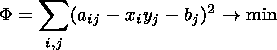(1)

where a_ij @. If there are any two known vectors, then the third one will be calculated through explicit formulas. As a result, for the given matrix A, we will find the best approximation, that is the matrix P₁. Further on, we look for a matrix, P₂, that is the best approximation of A-P₁ and so on, while the norm of A is not sufficiently close to zero. Thus, the initial matrix A is presented in the form of a sum of matrices of rank 1, that is, A=P₁+P₂+ +P_q. The Q factorial recovering of the gaps consists in their definition through the sum of matrices P_q. For incomplete data after a number of iterations, we get a system of factors that we will use for recovery. Further, we again construct a system of factors with the help of already recovered data and so on.

Figure 1

Geometrical interpretation of a linear model is shown in Figure 1a, for A R². We considered our example in R³ space, so our data point x is presented as (x₁,x₂,x₃). Imagine there is a point and that two of its coordinates are lost (we have only x₃ coordinate), so a plane, L_k, corresponds to it. The plane L_k is modeled by the vector y that is an inclined line approximating known data in a best manner; vector x is a set of projections of initial data on y (  M ). The lost coordinate now is substituted by the intersection L_k M.

Quasilinear models [Gorban et al., 2000; Rossiev, 1998] are based on the algorithm of linear model construction described above. First, we construct a linear model, then the vector-function f(t) (a cubic spline or a polynomial) that minimizes the functional:

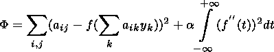(2)

where a>0 is a smoothing parameter.

So, first we are looking for the projection of data vector a on a manifold of small dimension y: Pr(a)=ty+b, t=(a,y), then we find a point on the curve f(t). For incomplete data, the closest point t(a) is taken on the manifold. And after that, we take the corresponding point on the curve f(t ) for t=t(a). After construction of f(t), the matrix A is substituted by the matrix of deviations from the model (Figure 1b). The process is repeated several times, and at the end the initial table, A is represented in a form of Q factorial model: a_iji,jf_i(t_j).

The third model is based on the Kohonen self-organizing maps theory or, more exactly, on the paradigm of self-organizing curves. These curves are defined by a set of points (a kernel) situated on a curve (at the first approach this curve is a polygonal one), on which a set of data point (taxon) must be mapped. Under fixed decomposition of the data set on taxons, the SOC is constructed uniquely. Under fixed location of kernels, taxons are easily constructed, too, with the help of minimizing of some functional, which consists of three addends: a measure of the best approximation, a measure of connectedness, and a measure of nonlinearity [Gorban et al., 2000]. Successive searching; kernels taxons kernels ... leads to the convergence of the algorithm. The computational process is implemented on the neural conveyor Famaster 2 made by Gorban's team at the Institute of Computational Mathematics of the Siberian Division of the Russian Academy of Sciences.

3. Results

Figure 2

Figure 3

Figure 4

We carried out the experiments with different time series. The results of some experiments are shown in Figure 2. About 50% of the points in the annual Wolf number time series were delete. For gap recovery, we used the SOC model. Strings of the initial data table were F. Takens m dimensional delay vectors [Sauer et al., 1991]. The time delay equals 1, and the embedding dimension equals 6. The strings look as follows: a_kj=x_k,x_k+1,...,x_k+5. The embedding dimension was estimated with the help of the False Nearest Neighbours' (FNN) method [Abarbanel et al., 1993]. Thus, deleting a point in a time series implied deleting the whole diagonal corresponding to that point. As you can see, the neural conveyor even recovered the peaks of cycles well. Figure 3 shows a fragment of the cosmogenic isotope ¹⁴C time series. The whole time series ranges from 5995 BC to 1945 AD. We give only the results recovering 30% of deleted points of the fragment from 5995 BC to 10 AD. And the last time series used in our experiment was ¹⁰Be (1428-1999 AD, annual data), and about 10% of points were deleted (Figure 4). Some results of recovery (in numerical form) are provided in Table 1. The construction of the initial table by F. Takens (unlike the arbitrary method of construction mentioned in Gorban et al. [[2000]; Rossiev [1998] essentially changes the situation. Really, a lost value of y component of the vector on Figure 1a induces a gap of x component in the next (by F. Takens) vector. The intersection of two lines recovers a missed value. In the multidimensional case, the problem is reduced to the search of a transverse intersection of hyperplanes [Sauer et al., 1991]. Thus, the method of gap recovery takes on a formal context.

3.1. Multifractal Spectrum of \boldmath ^<UNDEF>14 C Time Series

After applying the recovery procedure to the time series, we had an equidistant and complete one, so it became possible to use more refined tools to implement our investigations.

We used an approach in which time series is considered as multifractal random measures. Remember [Barreira et al. 1997] that multifractal spectrum of singularities of Borel finite measure m on a compact set X is a function f(a) defined by a pair (g,G). Here, g:X [-,+] is a function, which determines the level sets: g:K_a^g={x X:g(x)=a } and produces a multifractal decomposition X:

Let G be a real function, which is defined on Z_i X such that G(Z₁)2) if Z₁ Z₂. Then multifractal spectrum is f(a)=G(K_a^g). Let g be determined as pointwise dimension d_m of measure m at all points x X for which the limit

Figure 5

exists, where m(B(x,r)) is a "mass" of measure in the ball of radius r centered at x. Since we have chosen g=d_m, we can omit the subscript from further references to K_a^g. Then K_a={x:d_m(x)=a}, where the exponent is a local density of m. The singular distribution m can then be characterized by Hausdorff dimension of K_a, that is, f(a)=G(K_a)= dim_H(K_a). If m is self-similar in some sense, f(a) is a well-behaved concave function of f(a) [Falconer, 1994]. To estimate f(a), we applied the method of the partition sum [Riedi, 1997]. For analysis, annual ¹⁴C time series (1510-1954) was used. Initial time series had a fragment, where known data values were given in a period of 2 years (1890.5-1910.5), and there were some real data gaps (1911-1912, 1914, 1946). With the help of the method suggested above, this time series was recovered and became equidistant. Thus, the time series is applicable for multifractal analysis. In Figure 5, a f(a) -spectrum of this time series is shown. It shows that ¹⁴C records have multifractal properties in a large range of scales (1-2.2).

4. Conclusion

Our experiments have shown that the neural method for gap recovery in a time series is quite eligible for analyzing cosmogenic isotopes. This method allows equidistant time series to be obtained, which can be researched by using the modern tools of non-linear analysis.

References

Abarbanel, H. D. I., R. Brown, J. J. Sidorowich, and L. Sh. Tsimring, The analysis of observed chaotic data in physical systems, Rev. Mod. Phys., 65 (4), 1331, 1993.

Anderson, T. W., The Statistical Analysis of Time Series, Wiley, New York, 1971.

Bacry, E., J. F. Muzy, and A. Arnedo, Singularity spectrum of fractal signals from wavelet analysis: Exact results, J. Statist. Phys., 70 (3/4), 635, 1993.

Barreira, L., Y. Pesin, and J. Schmeling, On a general concept of multifractality: Multifractal spectra for dimensions, entropies, and Lyapunov exponents. Multifractal rigidity, Chaos, 7 (1), 27, 1997.

Davis, A., A. Marshak, W. Wiscombe, and R. Cahalan, Multifractal characterizations of nonstationarity and intermittence in geophysical fields: Observed, retrieved, or simulated, J. Geophys. Res., 99 (D4), 8055, 1994a.

Davis, A., A. Marshak, and W. Wiscombe, Wavelet-based multifractal analysis of nonstationary and/or intermittent geophysical signals, in Wavelets in Geophysics, edited by Efi Foufoula-Georgiou and Praveen Kumar, 249 pp., Academic Press, New York, 1994b.

Falconer, K. J., The Multifractal spectrum of statistically self-similar measures, J. Theor. Probab., 7 (3), 681, 1994.

Gorban, A. N., S. V. Makarov, and A. A. Rossiev, Neural conveyor to recover gaps in tables and construct regression by small samplings with incomplete data, Mathematics, Computer, Education (in Russian), 5 (II), 27, 1998.

Gorban, A. N., A. A. Rossiev, and D. C. Wunsch II, Self-organizing curves and neural modeling of data with gaps, Proceeding of Neuroinformatics 2000 (in Russian), Part 2, p. 40, Moscow, 2000.

Hastie, T., and W. Stuetzle, Principal curves, J. Am. Stat. Assoc., 84 (406), 502, 1988.

Kramer, M. A., Non-linear principal component analysis using autoassociative neural networks, AIChE J., 37 (2), 233, 1991.

Little, R. J. A., and D. B. Rubin, Statistical Analysis With Missing Data, John Wiley & Sons, Inc., New York, 1987.

MacDonald, G. J., Spectral analysis of time series generated by nonlinear processes, Rev. Geophys., 27 (4), 449, 1989.

Riedi, R. H., An Introduction to Multifractals, Rice University, 1997.

Rossiev, A. A., Modeling data by curves to recover the gaps in tables, Nueroinformatics Methods, 6, KGU Publishers, Krasnoyarsk, 1998.

Sauer, T., J. A. Yorke, and M. Casdagli, Embedology, J. Stat. Phys., 65 (3/4), 579, 1991.

Schreiber, T., Detecting and analyzing nonstationarity in time series using nonlinear cross predictions, Phys. Rev. Lett., 78 (5), 843, 1997.

Veneziano, D., Basic properties and characterization of stochastically self-similar processes, Rd. Fractal., 7 (1), 59, 1999.